5.11. Response surface methods

The purpose of response surface methods (RSM) is to optimize a process or system. RSM is a way to explore the effect of operating conditions (the factors) on the response variable, \(y\). As we map out the unknown response surface of \(y\), we move our process as close as possible towards the optimum, taking into account any constraints.

Initially, when we are far away from the optimum, we will use factorial experiments. As we approach the optimum then these factorials are replaced with better designs that more closely approximate conditions at the optimum.

Notice how it is a sequential approach. RSM then is a tool the describes how we should run these sequential sets of experiments. At the start of this section on designed experiments we showed how sequential experimentation (COST) leads to sub-optimal solutions. Why are we advocating sequential experimentation now? The difference is that here we use sequential experiments by changing multiple factors simultaneously, and not changing only one factor at a time.

RSM concept for a single variable: COST approach

We will however first consider just the effect of a single factor, \(x_1\) as it relates to our response, \(y\). This is to illustrate the general response surface process.

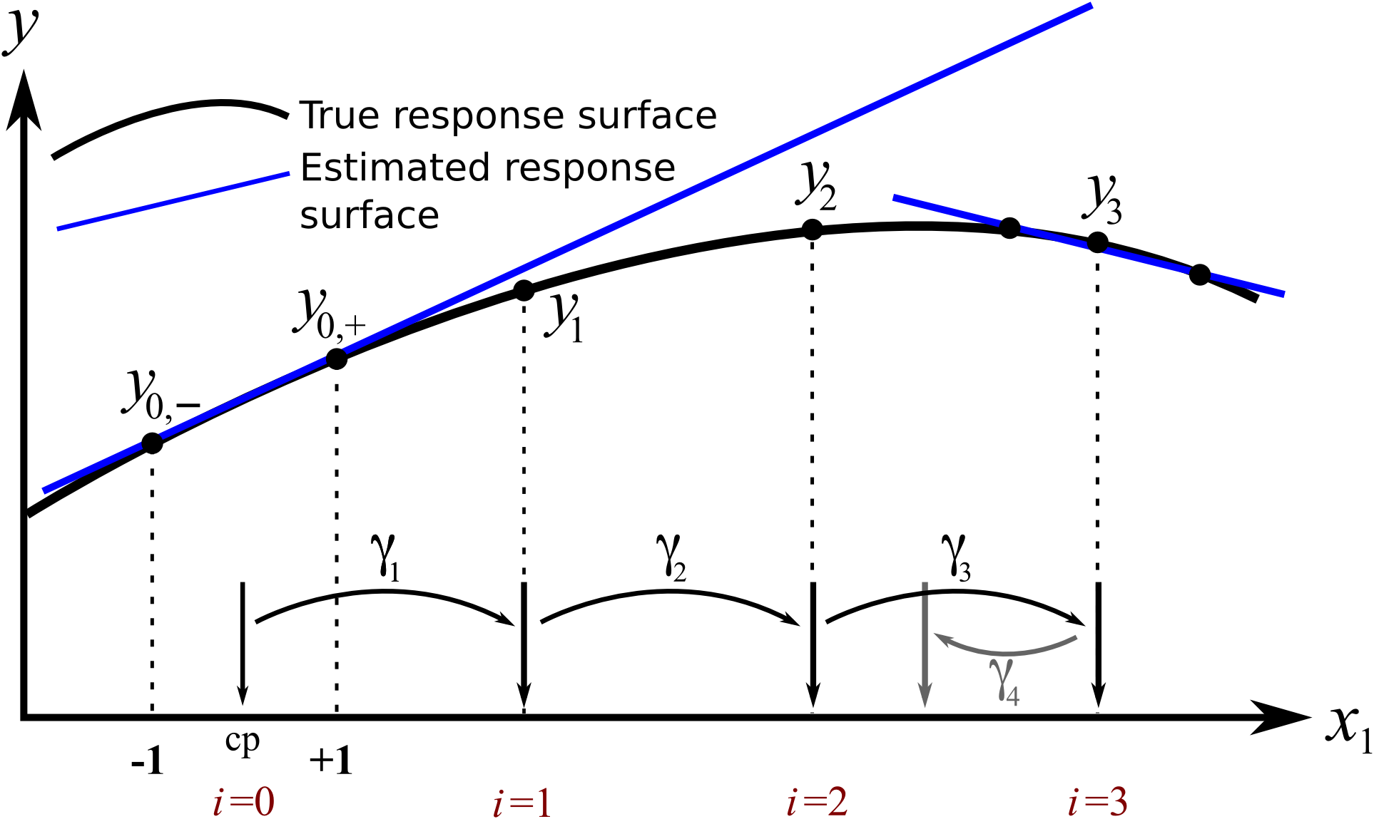
We start at the point marked \(i=0\) as our initial baseline (cp=center point). We run a 2-level experiment, above and below this baseline at \(-1\) and \(+1\), in coded units of \(x_1\), and obtain the corresponding response values of \(y_{0,-}\) and \(y_{0,+}\). From this we can estimate a best-fit straight line and move in the direction that increases \(y\). The sloping tangential line, also called the path of steepest ascent. Make a move of step-size = \(\gamma_1\) units along \(x_1\) and measure the response, recorded as \(y_1\). The response variable increased, so we keep going in this direction.

Make another step-size, this time of \(\gamma_2\) units in the direction that increases \(y\). We measure the response, \(y_2\), and are still increasing. Encouraged by this, we take another step of size \(\gamma_3\). The step-sizes, \(\gamma_i\) should be of a size that is big enough to cause a change in the response in a reasonable number of experiments, but not so big as to miss an optimum.

Our next value of \(y_3\) is about the same size as \(y_2\), indicating that we have plateaued. At this point we can take some exploratory steps and refit the tangential line (which now has a slope in the opposite direction). Or we can just use the accumulated points \(y = [y_{0-},\,\, y_{0+},\,\, y_1,\,\, y_2,\,\, y_3]\) and their corresponding \(x\)-values to fit a non-linear curve. Either way, we can then estimate a different step-size \(\gamma_4\) that will bring us closer to the optimum.

This univariate example is in fact what experimenters do when using the COST approach described earlier. We have:

• exploratory steps of different sizes towards an optimum

• refit the model once we plateau

• repeat

This approach works well if there really is only a single factor that affects the response. But with most systems there are multiple factors that affect the response. We show next how the exact same idea is used, only we change multiple variables at a time to find the optimum on the response surface.

5.11.1. Response surface optimization via a 2-variable system example

This example considers a new system here where two factors, temperature T, and substrate concentration S are known to affect the yield from a bioreactor. But in this example we are not just interested in yield, but actually the total profit from the system. This profit takes into account energy costs, raw materials costs and other relevant factors. The illustrations in this section show the contours of profit in light grey, but in practice these are obviously unknown.

We currently operate at this baseline condition:

• T = 325 K

• S = 0.75 g/L

• Profit = $407 per day

We start by creating a full factorial around this baseline by choosing \(\Delta_T = 10\) K, and \(\Delta_S = 0.5\) g/L based on our knowledge that these are sufficiently large changes to show an actual difference in the response value, but not too large so as to move to a totally different form of operation in the bioreactor.

The results from the full factorial are in the table here:

Experiment	T (actual)	S (actual)	T (coded)	S (coded)	Profit
Baseline	325 K	0.75 g/L	0	0	407
1	320 K	0.50 g/L	\(-\)	\(-\)	193
2	330 K	0.50 g/L	\(+\)	\(-\)	310
3	320 K	1.0 g/L	\(-\)	\(+\)	468
4	330 K	1.0 g/L	\(+\)	\(+\)	571

Clearly the promising direction to maximize profit is to operate at higher temperatures and higher substrate concentrations. But how much much higher and in what ratio should we increase \(T\) and \(S\)? These answers are found by building a linear model of the system from the factorial data:

\[\begin{split}\hat{y} &= b_0 + b_T x_T + b_S x_S + b_{TS} x_T x_S \\ \hat{y} &= 385.5 + 55 x_T + 134 x_S - 3.50 x_T x_S\end{split}\]

where \(x_T = \dfrac{x_{T,\text{actual}} - \text{center}_T}{\Delta_T / 2} = \dfrac{x_{T,\text{actual}} - 325}{5}\) and similarly, \(x_S = \dfrac{x_{S,\text{actual}} - 0.75}{0.25}\).

The model is fitted from the four corner runs (the centre run is held back to check for curvature later), and the coded design is orthogonal, so the coefficients are read straight off the corner responses:

Python, 16 lines

import numpy as np

# Coded corner design (standard order) and the measured profit.
xT = np.array([-1, +1, -1, +1])
xS = np.array([-1, -1, +1, +1])
profit = np.array([193, 310, 468, 571])

X = np.column_stack([np.ones(4), xT, xS, xT * xS])
b = np.linalg.solve(X.T @ X, X.T @ profit)
print(b)                       # -> [385.5, 55.0, 134.0, -3.5]

# Path of steepest ascent: move 1 coded unit in T, the ratio bS/bT in S,
# then unscale to real-world units using the half-ranges (5 K, 0.25 g/L).
dxS_coded = b[2] / b[1]         # 134 / 55
dS_actual = dxS_coded * 1 * 0.5 / 2
print(round(dS_actual, 2))     # -> 0.61 g/L per +5 K step in temperature

The model shows that we can expect an increase of $55/day of profit for a unit increase in \(x_T\) (coded units). In real-world units that would require increasing temperature by \(\Delta x_{T,\text{actual}} = (1) \times \Delta_T /2\) = 5K to achieve that goal. That scaling factor comes from the coding we used:

\[\begin{split}x_T &= \displaystyle \frac{x_{T,\text{actual}} - \text{center}_T}{\Delta_T / 2} \\ \Delta x_T &= \displaystyle \frac{\Delta x_{T,\text{actual}}}{\Delta_T / 2}\end{split}\]

Similarly, we can increase \(S\) by \(\Delta x_S = \text{1 unit} = 1 \times \Delta_S/2 = 0.5/2\) = 0.25 g/L real-world units, to achieve a $134 per day profit increase.

The interaction term is small, indicating the response surface is mostly linear in this region. The illustration shows the model’s contours (straight, green lines). Notice that the model contours are a good approximation to the actual contours (dotted, light grey), which are unknown in practice.

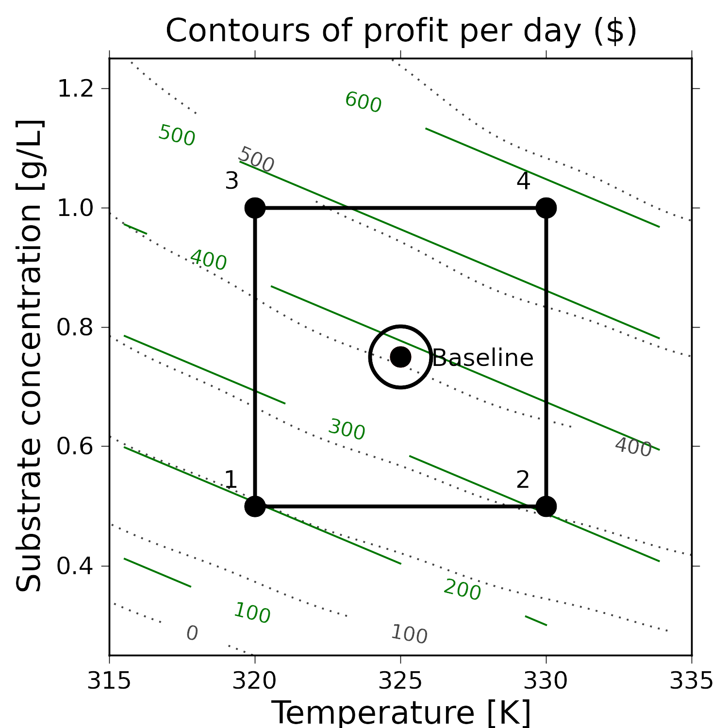
To improve our profit in the optimal way we move along our estimated model’s surface, in the direction of steepest ascent. This direction is found by taking partial derivatives of the model function, ignoring the interaction term, since it is so small.

\[\dfrac{\partial \hat{y}}{\partial x_T} = b_T = 55 \qquad \qquad \dfrac{\partial \hat{y}}{\partial x_S} = b_S = 134\]

This says for every \(b_T = 55\) coded units that we move by in \(x_T\) we should also move \(x_S\) by \(b_S = 134\) coded units. Mathematically:

\[\frac{\Delta x_S}{\Delta x_T} = \frac{134}{55}\]

The simplest way to do this is just to pick a move size in one of the variables, then change the move size of the other one.

So we will choose to increase \(\Delta x_T = 1\) coded unit, which means:

\[\begin{split} \Delta x_T &= 1 \\ \Delta x_{T,\text{actual}} &= 5 \,\text{K} \\ \Delta x_S &= \frac{b_S}{b_T} \Delta x_T = \frac{134}{55} \Delta x_T \\ \text{but we know that}\qquad\qquad \Delta x_S &= \frac{x_{S,\text{actual}}}{\Delta_S / 2} \\ \Delta x_{S,\text{actual}} &= \frac{134}{55} \times 1 \times \Delta_S / 2\,\, \text{by equating previous 2 lines} \\ \Delta x_{S,\text{actual}} &= \frac{134}{55} \times 1 \times 0.5 / 2 = \bf{0.61}\,\,\text{g/L}\\\end{split}\]

• \(T_5 = T_\text{baseline} + \Delta x_{T,\text{actual}} = 325 + 5 = 330\) K

• \(S_5 = S_\text{baseline} + \Delta x_{S,\text{actual}} = 0.75 + 0.61 = 1.36\) g/L

So when we run the next experiment at these conditions. The daily profit is \(y_5 =\) $ 669, improving quite substantially from the baseline case.

We decide to make another move, in the same direction of steepest ascent, i.e. along the vector that points in the \(\frac{134}{55}\) direction. We move the temperature up 5K, although we could have used a larger or smaller step size if we wanted:

• \(T_6 = T_5 + \Delta x_{T,\text{actual}} = 330 + 5 = 335\) K

• \(S_6 = S_5 + \Delta x_{S,\text{actual}} = 1.36 + 0.61 = 1.97\) g/L

Again, we determine profit at \(y_6 =\) $ 688. It is still increasing, but not by nearly as much. Perhaps we are starting to level off. However, we still decide to move temperature up by another 5 K and increase the substrate concentration in the required ratio:

• \(T_7 = T_6 + \Delta x_{T,\text{actual}} = 335 + 5 = 340\) K

• \(S_7 = S_6 + \Delta x_{S,\text{actual}} = 1.97 + 0.61 = 2.58\) g/L

The profit at this point is \(y_7 =\) $ 463. We have gone too far as profit has dropped off. So we return back to our last best point, because the surface has obviously changed, and we should refit our model with a new factorial in this neighbourhood:

Experiment	T (actual)	S (actual)	T	S	Profit
6	335 K	1.97 g/L	0	0	688
8	331 K	1.77 g/L	\(-\)	\(-\)	694
9	339 K	1.77 g/L	\(+\)	\(-\)	725
10	331 K	2.17 g/L	\(-\)	\(+\)	620
11	339 K	2.17 g/L	\(+\)	\(+\)	642

This time we have decided to use slightly smaller ranges in the factorial, \(\text{range}_T = 8 = (339 - 331)\) K and \(\text{range}_S = 0.4 = (2.17 - 1.77)\) g/L, so that we can move more slowly along the surface.

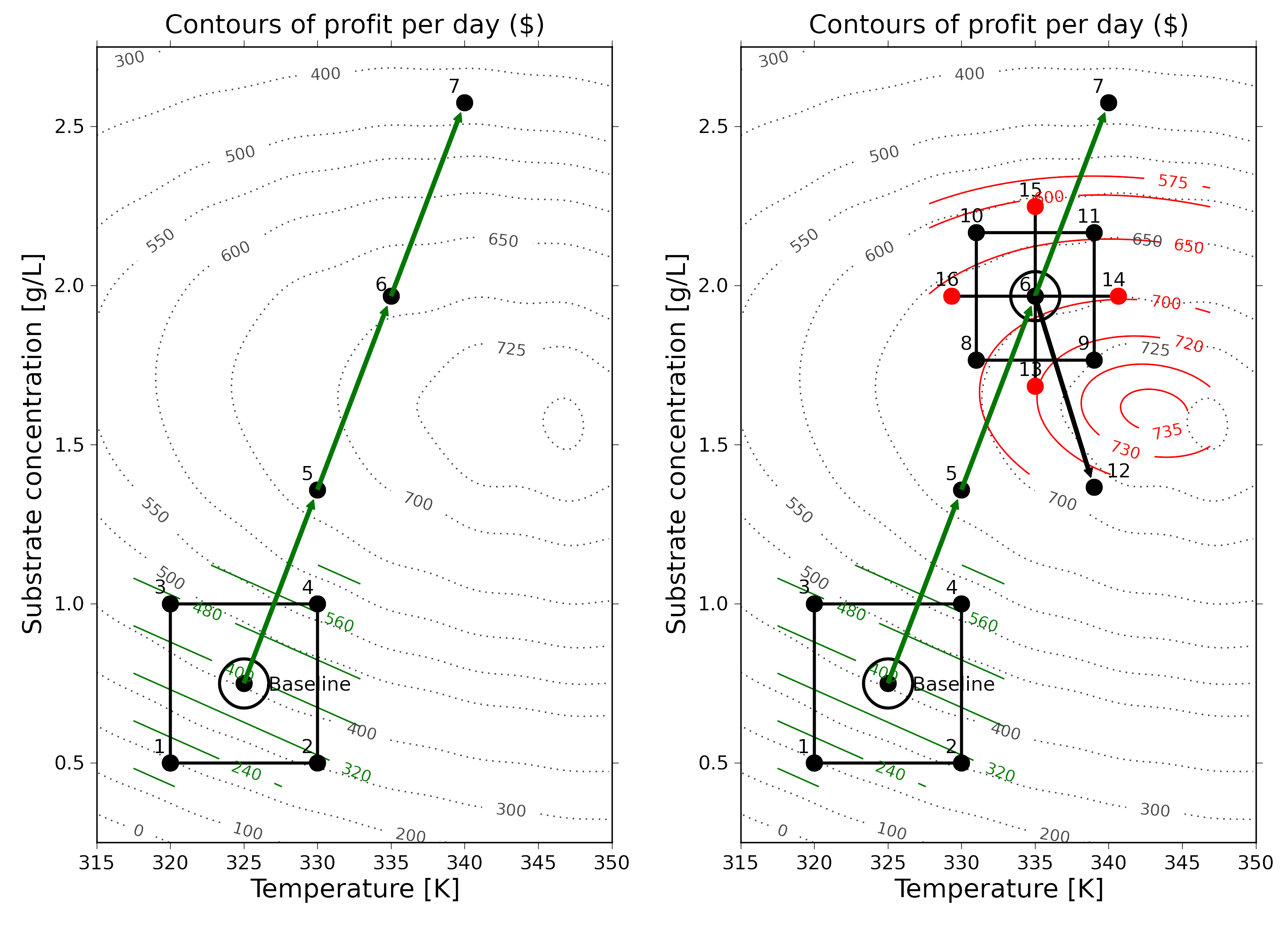
A least squares model from the 4 factorial points (experiments 8, 9, 10, 11, run in random order), seems to show that the promising direction now is to increase temperature but decrease the substrate concentration.

\[\begin{split}\hat{y} &= b_0 + b_T x_T + b_S x_S + b_{TS} x_T x_S \\ \hat{y} &= 670.25 + 13.25 x_T - 39.25 x_S - 2.25 x_T x_S\end{split}\]

As before we take a step in the direction of steepest ascent of \(b_T\) units along the \(x_T\) direction and \(b_S\) units along the \(x_S\) direction. Again we choose \(\Delta x_T = 1\) unit, though we must emphasize that we could used a smaller or larger amount, if desired.

\[\begin{split}\frac{\Delta x_S}{\Delta x_T} &= \frac{-39}{13} \\ \Delta x_S &= \frac{-39}{13} \times 1\\ \Delta x_{S, \text{actual}} &= \frac{-39}{13} \times 1 \times 0.4 /2 = -0.6\,\text{g/L}\\ \Delta x_{T, \text{actual}} &= 4\,\text{K}\\\end{split}\]

• \(T_{12} = T_6 + \Delta x_{T, \text{actual}}\) = 335 + 4 = 339K

• \(S_{12} = S_6 + \Delta x_{S, \text{actual}}\) = 1.97 - 0.6 = 1.37 g/L

We determine that at run 12 the profit is \(y_{12}\) = $ 716. But our previous factorial had a profit value of $725 on one of the corners. Now it could be that we have a noisy system; after all, the difference between $716 and $725 is not too much, but there is a relatively large difference in profit between the other points in the factorial.

One must realize that as one approaches an optimum we will find:

• The response variable will start to plateau, since, recall that the first derivative is zero at an optimum, implying the surface flattens out, and all points, in all directions away from the optimum are worse off.

• The response variable remains roughly constant for two consecutive jumps, because one has jumped over the optimum.

• The response variable decreases, sometimes very rapidly, because we have overshot the optimum.

• The two-factor interaction terms become similar to, or larger than, the main effect terms. This signals that the planar (first-order) model no longer describes the surface well: a large interaction warps the plane into a twisted surface. It is a warning that the first-order approximation is breaking down, though it is distinct from the pure quadratic curvature detected by the centre-point check below.

An optimum exhibits curvature, so a model that only has linear terms in it will not be suitable to use to find the direction of steepest ascent along the true response surface. We must add terms that account for this curvature.

Checking for curvature

The model above was fitted from the four corner runs only, so the centre run is held back as an independent check for curvature. The linear model predicts the centre from \((x_T, x_S) = (0, 0)\), which is just the intercept term. In the last factorial, the predicted centre point was \(\hat{y}_\text{cp}\) = $670.25; yet the actual centre point from run 6 showed a profit of $688. This is a difference of about $18, which is substantial when compared to the main effects’ coefficients, particularly of temperature.

So when the measured center point value is quite different from the predicted center point in the linear model, then that is a good indication there is curvature in the response surface. The way to accommodate for that is to add quadratic terms to the estimate model.

Adding higher-order terms using central composite designs

We will not go into too much detail about central composite designs, other than to show what they look like for the case of 2 and 3 variables. These designs take an existing orthogonal factorial and augment it with axial points. This is great, because we can start off with an ordinary factorial and always come back later to add the terms to account for nonlinearity.

The axial points are placed \(4^{0.25} = 1.4\) coded units away from the center for a 2 factor system, and \(8^{0.25} = 1.7\) units away for a \(k=3\) factor system. Rules for higher numbers of factors, and the reasoning behind the 1.4 and 1.7 unit step size can be found, for example in the textbook by Box, Hunter and Hunter.

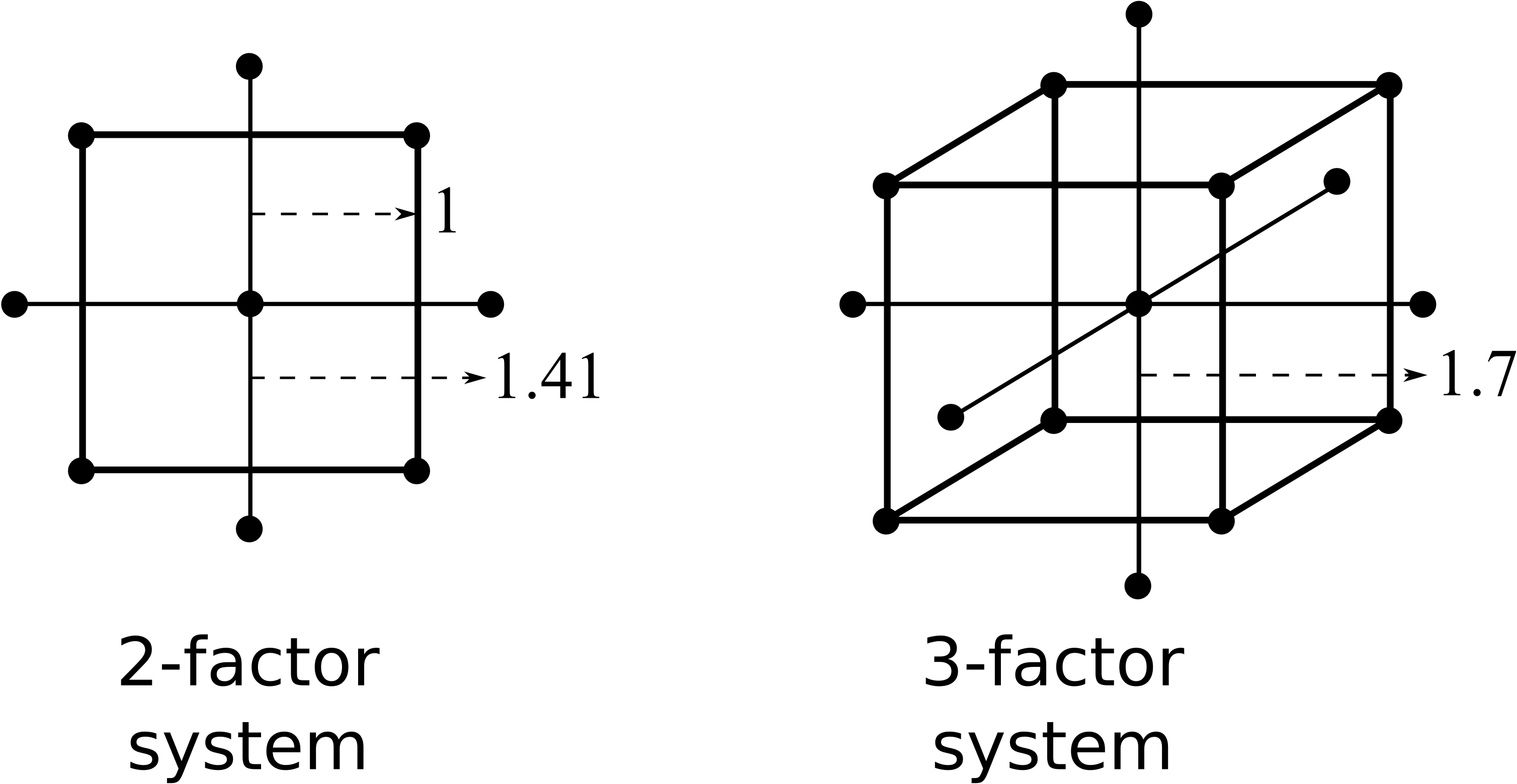
So a central composite design layout was added to the factorial in the above example and the experiments run, randomly, at the 4 axial points.

The four response values were \(y_{13} = 720\), \(y_{14} = 699\), \(y_{15} = 610\), and \(y_{16} = 663\). This allows us to estimate a model with quadratic terms in it: \(y = b_0 + b_T x_T + b_S x_S + b_{TS} x_T x_S + b_{TT} x_T^2 + b_{SS} x_S^2\). The parameters in this model are found in the usual way, using a least-squares model:

\[\begin{split}\mathbf{y} &= \mathbf{X} \mathbf{b} + \mathbf{e}\\ \begin{bmatrix} y_8\\ y_9\\ y_{10} \\ y_{11} \\ y_{6} \\ y_{13} \\ y_{14} \\ y_{15} \\ y_{16} \end{bmatrix} &= \begin{bmatrix} 1 & -1 & -1 & +1 & +1 & +1\\ 1 & +1 & -1 & -1 & +1 & +1\\ 1 & -1 & +1 & -1 & +1 & +1\\ 1 & +1 & +1 & +1 & +1 & +1\\ 1 & 0 & 0 & 0 & 0 & 0\\ 1 & 0 &-1.41& 0 & 0 & 2\\ 1 & 1.41& 0& 0 & 2 & 0\\ 1 & 0 & 1.41& 0 & 0 & 2\\ 1 &-1.41& 0& 0 & 2 & 0 \end{bmatrix} \begin{bmatrix} b_0 \\ b_T \\ b_S \\ b_{TS} \\ b_{TT} \\ b_{SS} \end{bmatrix} + \mathbf{e}\\ y &= 688 + 13x_T - 39x_S - 2.4 x_T x_S - 4.2 x_T^2 - 12.2 x_S^2\end{split}\]

Notice how the linear terms estimated previously are the same! The quadratic effects are clearly significant when compared to the other effects, which was what prevented us from successfully using a linear model to project out to point 12 previously.

The final step in the response surface methodology is to plot this model’s contour plot and predict where to run the next few experiments. As the solid contour lines in the illustration show, we should run our next experiments roughly at \(T\) = 343K and \(S\) = 1.60 g/L where the expected profit is around $736. We get those two values by eye-balling the solid contour lines, drawn from the above non-linear model. You could find this point analytically as well.

This is not exactly where the true process optimum is, but it is close to it (the temperature of \(T\) = 343 K is just a little lower than where the true optimum is).

This example has demonstrated how powerful response surface methods are. A minimal number of experiments has quickly converged onto the true, unknown process optimum. We achieved this by building successive least squares models that approximate the underlying surface. Those least squares models are built using the tools of fractional and full factorials and basic optimization theory, to climb the hill of steepest ascent.

5.11.2. Checking the fit: pure error and the lack-of-fit test

Once a quadratic model is fitted, a natural question is whether it actually describes the surface, or whether it is still missing a term. Comparing a predicted centre point against its measured value, as done above, is an informal version of this check. With replicated runs it can be made into a formal test.

The idea is to split the model’s residual sum of squares into two parts. Replicated runs, meaning two or more runs at exactly the same factor-level combination, differ only by noise, so the spread among their responses estimates the pure error: the run-to-run variability of the system, without reference to any model. Writing \(Y_{ij}\) for the \(j\)-th response at the \(i\)-th replicated combination, \(\bar{Y}_i\) for its average, \(m\) for the number of replicated combinations, and \(n_i\) for the number of replicates there, the pure-error sum of squares is

\[\text{SS}_\text{PE} = \sum_{i=1}^{m} \sum_{j=1}^{n_i} \left(Y_{ij} - \bar{Y}_i\right)^2 .\]

Whatever is left of the residual sum of squares \(\text{SS}_\text{E}\) is the lack-of-fit sum of squares,

\[\text{SS}_\text{LOF} = \text{SS}_\text{E} - \text{SS}_\text{PE},\]

which measures the part of the residual that the model failed to explain but that is not just noise. The degrees of freedom split the same way: with \(n\) runs and \(p\) parameters the residual carries \(n - p\), the pure error carries \(\text{df}_\text{PE} = \sum_i (n_i - 1)\), and the lack of fit carries the remainder, \(\text{df}_\text{LOF} = n - p - \text{df}_\text{PE}\).

If the model is adequate, the lack-of-fit and pure-error mean squares both estimate the same noise variance, so their ratio

\[F = \frac{\text{SS}_\text{LOF} / \text{df}_\text{LOF}}{\text{SS}_\text{PE} / \text{df}_\text{PE}}\]

follows an \(F\)-distribution with \(\text{df}_\text{LOF}\) and \(\text{df}_\text{PE}\) degrees of freedom. A large \(F\), with a small \(p\)-value, is evidence that the model is missing a term (often a higher-order effect). For example, a 15-run experiment fitting an 8-parameter model, with two combinations each run twice, has \(\text{df}_\text{PE} = (2-1) + (2-1) = 2\) and \(\text{df}_\text{LOF} = 15 - 8 - 2 = 5\). An \(F\)-ratio near 3 there carries a \(p\)-value of about 0.27, which gives no reason to doubt the model. The test needs both replicated points (to get \(\text{SS}_\text{PE}\)) and more distinct design points than parameters (to leave some \(\text{df}_\text{LOF}\)).

5.11.3. Box-Behnken designs

A Box-Behnken design (BBD) is a three-level (\(-1, 0, +1\)) response surface design that supports the same full second-order (quadratic) model as the central composite design above. Box and Behnken (1960) constructed them by combining two-level factorials with balanced incomplete block designs. Each non-centre run sits at the midpoint of an edge of the experimental cube: two factors are set to their extremes (a \(2 \times 2\) factorial in that pair) while all the remaining factors are held at the centre. Centre points are then replicated, to estimate the pure error and to stabilise the prediction near the middle of the region.

The defining feature. A BBD places no runs at the cube vertices: there is no run with every factor simultaneously at its high or low setting. All the design points lie on a sphere of radius \(\sqrt{2}\) in coded units (the edge midpoints), plus the centre. This single property is what separates a BBD from a central composite design (CCD), and it drives every practical consequence. Because the extreme corner combinations are never required, a BBD is attractive when the corners of the region are infeasible, unsafe, or physically meaningless: high temperature with high pressure and high concentration all at once, for example. It also keeps each factor at three operationally convenient settings, which simplifies the execution.

A BBD has these properties:

• it fits the full quadratic model: intercept, linear, two-factor interaction, and pure quadratic terms;

• it requires at least three factors, and does not exist for two;

• it is rotatable for \(k = 4\) (and \(k = 7\)), and nearly rotatable for the other factor counts, including \(k = 3\), giving roughly uniform prediction variance at a fixed distance from the centre;

• it is spherical rather than cuboidal: the prediction quality is good in the interior, and degrades towards the corners, where there is no design support.

The run count, and how it compares with a rotatable CCD, is what usually decides the matter in practice.

Run counts for a Box-Behnken design.

Factors \(k\)	Edge points	Centre points (typical)	Total runs
3	12	3	15
4	24	3	27
5	40	6	46
6	48	6	54
7	56	6	62

Box-Behnken compared with central composite designs.

Aspect	Box-Behnken	Central composite
Factor levels	3	5 (rotatable) or 3 (face-centred)
Corner runs	none	yes (the factorial portion)
Region shape	spherical	spherical or cuboidal
Runs at \(k = 3\)	15	about 20
Sequential build	no	yes: augment a factorial with axial and centre points
Prediction at corners	weak	strong

For three and four factors a BBD is usually more economical than a rotatable CCD. The trade-off is that a BBD cannot be assembled sequentially from a screening factorial, and it should not be used when the corner conditions are themselves of interest, since the model is effectively extrapolating there.

Where they are used. Box-Behnken designs are an optimisation-stage tool, reached once screening has reduced the factor set to roughly three to five important continuous factors. They are common in analytical method development and analytical quality by design (HPLC and other separations), in pharmaceutical formulation and quality by design, in fermentation and bioprocess optimisation, in extraction, and in food and beverage science. In each case the appeal is the same: a compact second-order design that never asks for the dangerous or impossible corner of the operating space.

There are three situations where a BBD is the wrong choice:

• with only two factors, or when the corner conditions must be explored: use a CCD, or a face-centred CCD;

• when a sequential path from screening to response surface modelling is planned: a CCD augments a factorial directly, whereas a BBD does not;

• with categorical factors, or hard constraints on the region: prefer an optimal (D- or I-) design.

Readings

• Box, G.E.P. and Behnken, D.W.: “Some New Three Level Designs for the Study of Quantitative Variables”, Technometrics, 2, 455–475, 1960. doi:10.1080/00401706.1960.10489912

• Myers, Montgomery and Anderson-Cook, Response Surface Methodology, the chapter on second-order designs; and Montgomery, Design and Analysis of Experiments, the response surface chapter.

5.11.4. The general approach for response surface modelling

1. Start at your baseline conditions and identify the main factors based on physics of the process, operator input, expert opinion input, and intuition. Also be aware of any constraints, especially for safe process operation. Perform factorial experiments (full or fractional factorials), completely randomized. Use the results from the experiment to estimate a linear model of the system:

   \[\hat{y} = b_0 + b_Ax_A + b_B x_B + b_C x_C \ldots + b_{AB}x_Ax_B + b_{AC} x_A x_C + \ldots\]

2. Far from the optimum the main effects are usually larger than the two-factor interactions. When that holds, the interaction terms are small enough to leave out of the direction calculation in the next step. Check it rather than assume it: if an interaction is comparable to or larger than the main effects, the simple gradient step below does not apply (see the note after this list). Any main effects that are not significant may be dropped for future iterations.

3. Use the model to estimate the path of steepest ascent (or descent if minimizing \(y\)):

   \[\dfrac{\partial \hat{y}}{\partial x_1} = b_1 \qquad\qquad \dfrac{\partial \hat{y}}{\partial x_2} = b_2 \qquad \ldots\]

   The path of steepest ascent is climbed. Move any one of the main effects, e.g. \(b_A\) by a certain amount, \(\Delta x_A\). Then move the other effects: \(\Delta x_i = \frac{b_i}{b_A} \Delta x_A\). For example, \(\Delta x_C\) is moved by \(\frac{b_C}{b_A} \Delta x_A\).

   This simple ratio is the gradient of the first-order (planar) part of the model, so it points along the steepest ascent only while the interaction terms are negligible. If the two-factor interactions are similar to, or larger than, the main effects, the fitted surface is a twisted plane rather than a flat one, and the direction of steepest ascent turns as you move. In that case, do not follow the linear gradient blindly: draw the contour plot of the fitted model and read the next point off the surface, or move to a second-order design (central composite design) that can describe the curvature.

   If any of the \(\Delta x_i\) values are too large to safely implement, then take a smaller proportional step in all factors. Recall that these are coded units, so unscale them to obtain the move amount in real-world units.

4. One can make several sequential steps until the response starts to level off, or if you become certain you have entered a different operating mode of the process.

5. At this point you repeat the factorial experiment from step 1, making the last best response value your new baseline. This is also a good point to reintroduce factors that you may have omitted earlier. Also, if you have a binary factor; investigate the effect of alternating its sign at this point. These additional factorial experiments should also include center points.

6. Repeat steps 1 through 5 until the linear model estimate starts to show evidence of curvature, or that the interaction terms start to dominate the main effects. This indicates that you are reaching an optimum.

   • Curvature can be assessed by comparing the predicted center point, i.e. the model’s intercept = \(b_0\), against the actual center point response(s). A large difference in the prediction, when compared to the model’s effects, indicates the response surface is curved.

7. If there is curvature, add axial points to expand the factorial into a central composite design. Now estimate a quadratic model of the form:

   \[y = b_0 + b_1x_1 + b_2 x_2 + \ldots + b_{12}x_1x_2 + \ldots + b_{11}x_1^2 + b_{22}x_2^2 + \ldots\]

8. Draw contour plots of this estimated response surface (all data analysis software packages have contour plotting functions) and determine where to place your sequential experiments. You can also find the model’s optimum analytically by taking derivatives of the model function.

What is the response variable when optimizing more than one outcome?

Response surface methods consider optimization of a single outcome, or response variable, called \(y\). In many instances we are interested in just a single response, but more often we are interested in a multi-objective response, i.e. there are trade-offs. For example we can achieve a higher production rate, but it is at the expense of more energy.

One way to balance all competing objectives is to rephrase the \(y\) variable in terms of total costs, or better still, net profit. This makes calculating the \(y\) value more complex, as we have to know the various costs and their relative weightings to calculate the profit. Now you have a single \(y\) to work with. That is the route taken in the bioreactor example throughout this section.

Another way is to superimpose the response surfaces of two or more \(y\)-variables. This is tremendously helpful when discussing and evaluating alternate operating points, because plant managers and operators can then visually see the trade-offs.

Both routes, and a third that grades each response and optimizes the combination, are covered in the section on multi-response optimization, which continues this same bioreactor example with a second response measured alongside profit.

Summary

1. In the previous sections we used factorials and fractional factorials for screening the important factors. When we move to process optimization, we are assuming that we have already identified the important variables. In fact, we might find that variables that were previously important, appear unimportant as we approach the optimum. Conversely, variables that might have been dropped out earlier, become important at the optimum.

2. Response surface methods generally work best when the variables we adjust are numerically continuous. Categorical variables (yes/no, catalyst A or B) are handled by fixing them at one or the other value, and then performing the optimization conditional on those selected values. It is always worth investigating the alternative values once the optimum has been reached.

3. Many software packages provide tools that help with an RSM study. If you would like to use R in your work, we highly recommend the rsm package by Russel Lenth, available in R. You can read more about the package in this article as well as a case-study.

5.12. Evolutionary operation

Evolutionary operation (EVOP) is a tool to help maintain a full-scale process at its optimum. Since the process is not constant, the optimum will gradually move away from its current operating point. Chemical processes drift due to things such as heat-exchanger fouling, build-up inside reactors and tubing, catalyst deactivation, and other slowly varying disturbances in the system.

EVOP is an iterative hunt for the process optimum by making small perturbations to the system. Similar to response surface methods, once every iteration is completed, the process is moved towards the optimum. The model used to determine the move direction and levels of next operation are from full or fractional factorials, or designs that estimate curvature, like the central composite design.

Because every experimental run is a run that is expected to produce saleable product (we don’t want off-specification product), the range over which each factor is varied must be small. Replicate runs are also made to separate the signal from noise, because the optimum region is usually flat.

Some examples of the success of EVOP and a review paper are in these readings:

• George Box: Evolutionary Operation: A Method for Increasing Industrial Productivity”, Journal of the Royal Statistical Society (Applied Statistics), 6, 81 - 101, 1957.

• William G. Hunter and J. R. Kittrell, “Evolutionary Operation: A Review”, Technometrics, 8, 389-397, 1966.

Current day examples of EVOP do not appear in the scientific literature much, because this methodology is now so well established.