5.8.4. Analysis by least squares modelling

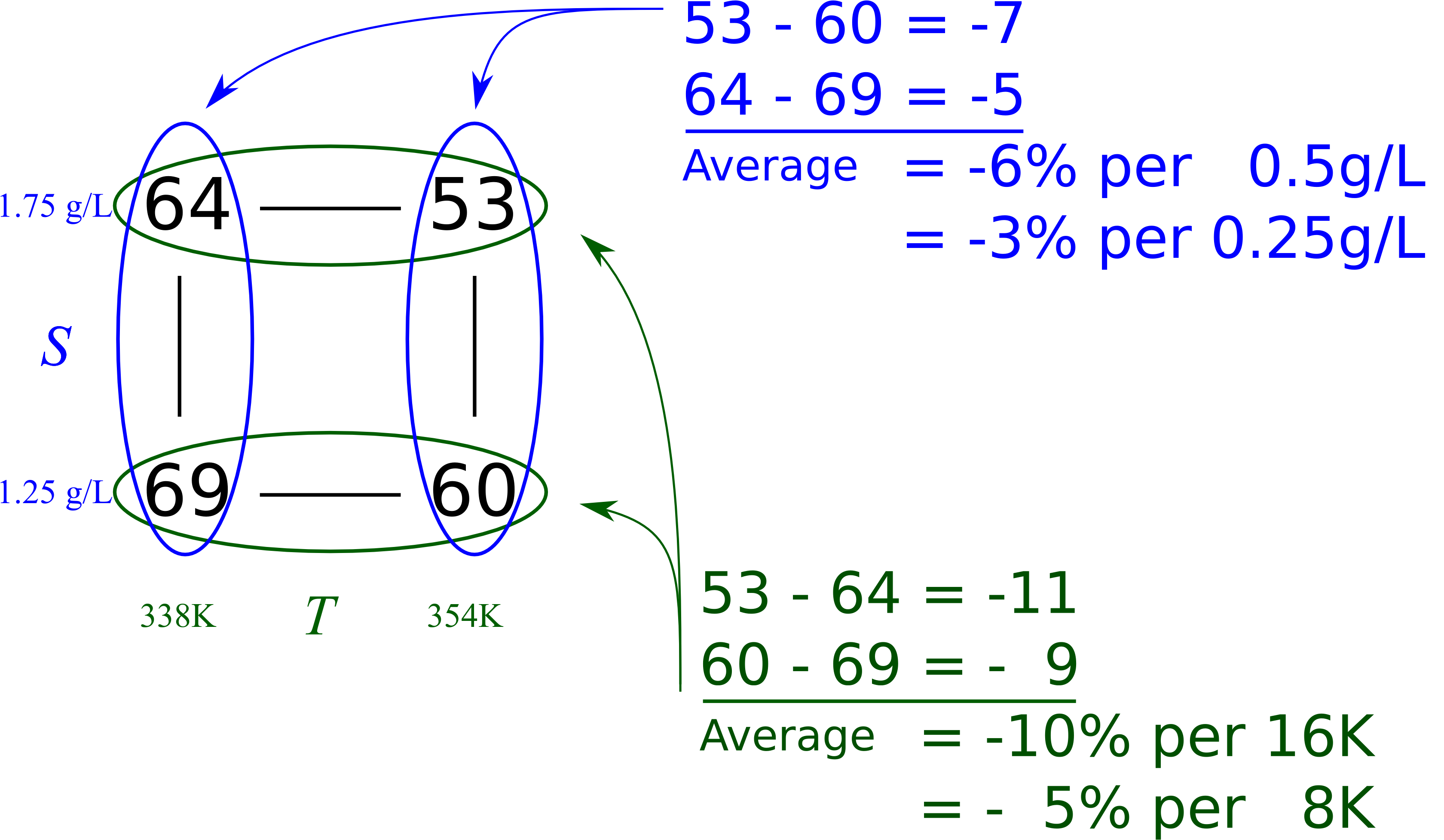
Let’s review the original system (the one with little interaction) and analyze the experimental data using a least squares model. We represent the original data here, with the baseline conditions:

Experiment

\(T\) [K]

\(S\) [g/L]

\(y\) [%]

Baseline

346 K

1.50

1

\(-\) (338 K)

\(-\) (1.25 g/L)

69

2

\(+\) (354 K)

\(-\) (1.25 g/L)

60

3

\(-\) (338 K)

\(+\) (1.75 g/L)

64

4

\(+\) (354 K)

\(+\) (1.75 g/L)

53

It is standard practice to represent the data from designed experiments in a centered and scaled form: \(\dfrac{\text{variable} - \text{center point}}{\text{range}/2}\). This gives the following values:

  • \(T_{-} = \dfrac{338 - 346}{(354-338)/2} = \dfrac{-8}{8} = -1\)

  • \(S_{-} = \dfrac{1.25 - 1.50}{(1.75 - 1.25)/2} = \dfrac{-0.25}{0.25} = -1\)

Similarly, \(T_{+} = +1\) and \(S_{+} = +1\), while the center points (baseline experiment) would be \(T_{0} = 0\) and \(S_{0} = 0\).

We will propose a least squares model that describes this system:

\[\begin{split}\text{Population model}: \qquad\qquad &y = \beta_0 + \beta_Tx_T + \beta_S x_S + \beta_{TS} x_Tx_S + \varepsilon\\ \text{Sample model}: \qquad\qquad &y = b_0 + b_Tx_T + b_S x_S + b_{TS} x_Tx_S + e\\\end{split}\]

We have four parameters to estimate and four data points. This means when we fit the model to the data, we will have no residual error, because there are no degrees of freedom left. If we had replicate experiments, we would have degrees of freedom to estimate the error, but more on that later. Writing the above equation for each observation,

\[\begin{split}\begin{bmatrix} y_1\\ y_2\\ y_3 \\ y_4 \end{bmatrix} &= \begin{bmatrix} 1 & T_{-} & S_{-} & T_{-}S_{-}\\ 1 & T_{+} & S_{-} & T_{+}S_{-}\\ 1 & T_{-} & S_{+} & T_{-}S_{+}\\ 1 & T_{+} & S_{+} & T_{+}S_{+}\\ \end{bmatrix} \begin{bmatrix} b_0 \\ b_T \\ b_S \\ b_{TS} \end{bmatrix} + \begin{bmatrix} e_1\\ e_2\\ e_3 \\ e_4 \end{bmatrix} \\ \begin{bmatrix} 69\\ 60\\ 64\\ 53 \end{bmatrix} &= \begin{bmatrix} 1 & -1 & -1 & +1\\ 1 & +1 & -1 & -1\\ 1 & -1 & +1 & -1\\ 1 & +1 & +1 & +1\\ \end{bmatrix} \begin{bmatrix} b_0 \\ b_T \\ b_S \\ b_{TS} \end{bmatrix} + \begin{bmatrix} e_1\\ e_2\\ e_3 \\ e_4 \end{bmatrix}\\ \mathbf{y} &= \mathbf{X} \mathbf{b} + \mathbf{e}\end{split}\]

Where the last line is a more compact representation. Notice then that the matrices from linear regression are:

\[\begin{split}\mathbf{X}^T\mathbf{X} &= \begin{bmatrix} 4 & 0 & 0 & 0\\ 0 & 4 & 0 & 0\\ 0 & 0 & 4 & 0\\ 0 & 0 & 0 & 4 \end{bmatrix} \\ \mathbf{X}^T\mathbf{y} &= \begin{bmatrix} 246 \\ -20 \\ -12 \\ -2\end{bmatrix} \\ \mathbf{b} = (\mathbf{X}^T\mathbf{X})^{-1}\mathbf{X}^T\mathbf{y} &= \begin{bmatrix} 1/4 & 0 & 0 & 0\\ 0 & 1/4 & 0 & 0\\ 0 & 0 & 1/4 & 0\\ 0 & 0 & 0 & 1/4 \end{bmatrix} \begin{bmatrix} 246 \\ -20 \\ -12 \\ -2\end{bmatrix}= \begin{bmatrix} 61.5 \\ -5 \\ -3 \\ -0.5 \end{bmatrix}\\\end{split}\]

Some things to note are (1) the orthogonality of \(\mathbf{X}^T\mathbf{X}\) and (2) the interpretation of these coefficients.

  1. Note how the \(\mathbf{X}^T\mathbf{X}\) matrix has only zeros on the off-diagonals: it indicates that matrix \(\mathbf{X}\) is orthogonal and confirms, algebraically, what we knew intuitively. The change we made in temperature, \(T\), was independent of the changes we made in substrate concentration, \(S\). This means that we can separately calculate and interpret the slope coefficients in the model.

  2. What is the interpretation of, for example, \(b_T = -5\)? Recall, from the section on linear regression interpretation, that it is the effect of increasing the temperature by 1 unit. In this case, the \(x_T\) variable has been normalized, but this slope coefficient represents the effect of changing \(x_T\) from 0 to 1, which in the original units of the variables is a change from 346 to 354 K, that is, an 8 K increase in temperature. It equally well represents the effect of changing \(x_T\) from \(-1\) to 0: a change from 338 K to 346 K decreases conversion by 5%.

    Similarly, the slope coefficient for \(b_S = -3\) represents the expected decrease in conversion when \(S\) is increased from 1.50 g/L to 1.75 g/L.

    Now contrast these numbers with those in the graphical analysis done previously and repeated below. They are the same, as long as we are careful to interpret them as the change over half the range.

    ../../_images/factorial-two-levels-two-variables-with-analysis.png

    The 61.5 term in the least squares model is the expected conversion at the baseline conditions. Notice from the least squares equations how it is just the average of the four experimental values, even though we did not actually perform an experiment at the center.

Let’s return to the system with high interaction where the four outcome values in standard order were 77, 79, 81 and 89. Looking back, the baseline operation was \(T\) = 395 K and \(S = \frac{1.25 - 0.5}{2}\) = 0.875 g/L; you should prove to yourself that the least squares model is

\[y = 81.5 + 2.5 x_T + 3.5 x_S + 1.5 x_T x_S\]

The interaction term can now be readily interpreted: it is the additional increase in conversion seen when both temperature and substrate concentration are at their high level. If \(T\) is at the high level and \(S\) is at the low level, then the least squares model shows that conversion is expected at \(81.5 + 2.5 - 3.5 - 1.5 = 79\). The interaction term has decreased conversion by 1.5 units.

fake width

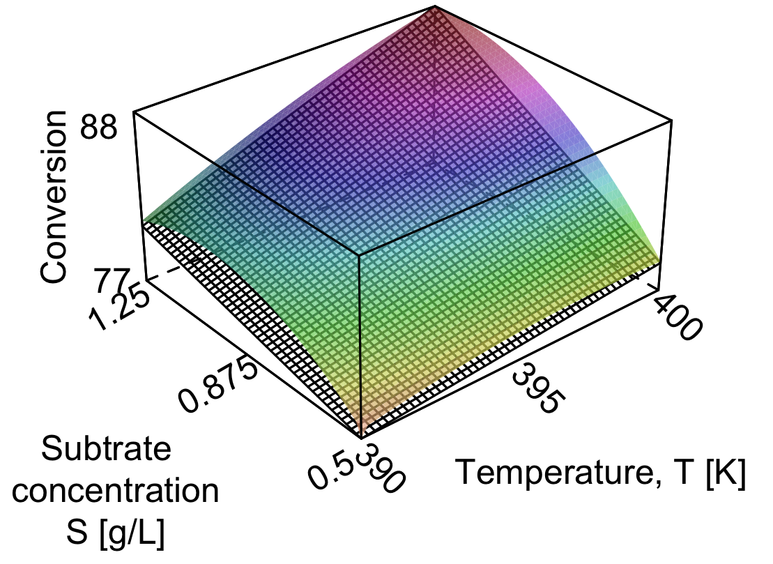
Finally, out of interest, the nonlinear surface that was used to generate the experimental data for the interacting system is coloured in the illustration. In practice we never know what this surface looks like, but we estimate it with the least squares plane, which appears below the nonlinear surface as black and white grids. The corners of the box are outer levels at which we ran the factorial experiments.

The corner points are exact with the nonlinear surface, because we have used the four values to estimate four model parameters. There are no degrees of freedom left, and the model’s residuals are therefore zero. Obviously, the linear model will be less accurate away from the corner points when the true system is nonlinear, but it is a useful model over the region in which we will use it later in the section on response surface methods.