
 Download PDF of entire book
6.5.16. Determining the number of components to use in the model with cross-validation
Cross-validation is a general tool that helps to avoid over-fitting - it can be applied to any model, not just latent variable models.
As we add successive components to a model we are increasing the size of the model, \(A\), and we are explaining the model-building data, \(\mathbf{X}\), better and better. (The equivalent in least squares models would be to add additional \(\mathbf{X}\)-variable terms to the model.) The model’s \(R^2\) value will increase with every component. As the following equation shows, the variance of the \(\widehat{\mathbf{X}}\) matrix increases with every component, while the residual variance in matrix \(\mathbf{E}\) must decrease.
This holds for any model where the \(\widehat{\mathbf{X}}\) and \(\mathbf{E}\) matrices are completely orthogonal to each other: \(\widehat{\mathbf{X}}'\mathbf{E} = \mathbf{0}\) (a matrix of zeros), such as in PCA, PLS and least squares models.
There comes a point for any real data set where the number of components, \(A\) = the number of columns in \(\mathbf{T}\) and \(\mathbf{P}\), extracts all systematic variance from \(\mathbf{X}\), leaving unstructured residual variance in \(\mathbf{E}\). Fitting any further components will start to fit this noise, and unstructured variance, in \(\mathbf{E}\).
Cross-validation for multivariate data sets was described by Svante Wold in his paper on Cross-validatory estimation of the number of components in factor and principal components models, in Technometrics, 20, 397-405, 1978.
For a critical review of cross-validation procedures applied to component models, see Bro, Kjeldahl, Smilde and Kiers (2008), Cross-validation of component models: A critical look at current methods.
The general idea is to divide the matrix \(\mathbf{X}\) into \(G\) groups of rows. These rows should be selected randomly, but are often selected in order: row 1 goes in group 1, row 2 goes in group 2, and so on. We can collect the rows belonging to the first group into a new matrix called \(\mathbf{X}_{(1)}\), and leave behind all the other rows from all other groups, which we will call group \(\mathbf{X}_{(-1)}\). So in general, for the \(g^\text{th}\) group, we can split matrix \(\mathbf{X}\) into \(\mathbf{X}_{(g)}\) and \(\mathbf{X}_{(-g)}\).
A row-wise cross-validation procedure asks to build the PCA model on the data in \(\mathbf{X}_{(-1)}\) using \(A\) components. Then use data in \(\mathbf{X}_{(1)}\) as new, testing data. In other words, we preprocess the \(\mathbf{X}_{(1)}\) rows, calculate their score values, \(\mathbf{T}_{(1)} = \mathbf{X}_{(1)} \mathbf{P}\), calculate their predicted values, \(\widehat{\mathbf{X}}_{(1)} = \mathbf{T}_{(1)} \mathbf{P'}\), and their residuals, \(\mathbf{E}_{(1)} = \mathbf{X}_{(1)} - \widehat{\mathbf{X}}_{(1)}\). We repeat this process, building the model on \(\mathbf{X}_{(-2)}\) and testing it with \(\mathbf{X}_{(2)}\), to eventually obtain \(\mathbf{E}_{(2)}\).
After repeating this on \(G\) groups, we gather up \(\mathbf{E}_{1}, \mathbf{E}_{2}, \ldots, \mathbf{E}_{G}\) and assemble a type of residual matrix, \(\mathbf{E}_{A,\text{CV}}\), where the \(A\) represents the number of components used in each of the \(G\) PCA models. The \(\text{CV}\) subscript indicates that this is not the usual error matrix, \(\mathbf{E}\). From this we can calculate a type of \(R^2\) value. We don’t call this \(R^2\), but it follows the same definition for an \(R^2\) value. We will call it \(Q^2_A\) instead, where \(A\) is the number of components used to fit the \(G\) models.
We also calculate the usual PCA model on all the rows of \(\mathbf{X}\) using \(A\) components, then calculate the usual residual matrix, \(\mathbf{E}_A\). This model’s \(R^2\) value is:
The \(Q^2_A\) behaves exactly as \(R^2\), but with two important differences. Like \(R^2\), it is a number less than 1.0 that indicates how well the testing data, in this case testing data that was generated by the cross-validation procedure, are explained by the model. The first difference is that \(Q^2_A\) is always less than the \(R^2\) value. The other difference is that \(Q^2_A\) will not keep increasing with each successive component, it will, after a certain number of components, start to decrease. This decrease in \(Q^2_A\) indicates the new component just added is not systematic: it is unable to explain the cross-validated testing data. We often see plots such as this one:
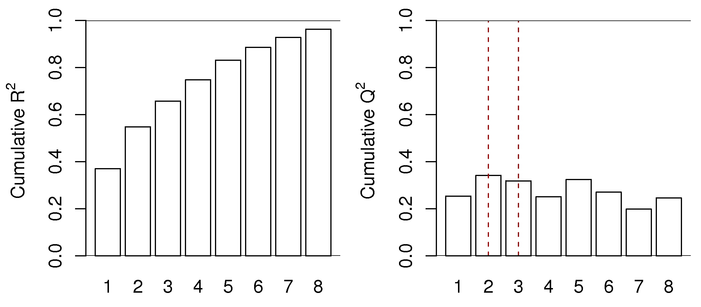
This is for a real data set, so the actual cut off for the number of components could be either \(A =2\) or \(A=3\), depending on what the 3rd component shows to the user and how interested they are in that component. Likely the 4th component, while boosting the \(R^2\) value from 66% to 75%, is not really fitting any systematic variation. The \(Q^2\) value drops from 32% to 25% when going from component 3 to 4. The fifth component shows \(Q^2\) increasing again. Whether this is fitting actual variability in the data or noise is for the modeller to determine, by investigating that 5th component. These plots show that for this data set we would use between 2 and 5 components, but not more.
Cross-validation, as this example shows is never a precise answer to the number of components that should be retained when trying to learn more about a dataset. Many studies try to find the “true” or “best” number of components. This is a fruitless exercise; each data set means something different to the modeller and the objective for which the model was intended to assist.
The number of components to use should be judged by the relevance of each component. Use cross-validation as guide, and always look at a few extra components and step back a few components; then make a judgement that is relevant to your intended use of the model.
However, cross-validation’s objective is useful for predictive models, such as PLS, so we avoid over-fitting components. Models where we intend to learn from, or optimize, or monitor a process may well benefit from fewer or more components than suggested by cross-validation.
A caution: do not reconstruct a left-out row from its own values. The procedure above projects each held-out row onto the loadings, \(\mathbf{T}_{(g)} = \mathbf{X}_{(g)} \mathbf{P}\), and then reconstructs that same row from those scores. The scores used to predict the row are therefore calculated from the very values we are trying to predict. As more components are added the loadings span more of the measurement space, so the cross-validated reconstruction error tends to keep shrinking even when the extra component is not real. As the number of components, \(A\), approaches the number of variables, \(K\), the held-out row is reproduced almost perfectly and \(Q^2_A\) becomes too optimistic. The effect is strongest when there are few variables, which is exactly the situation in the small example above.
This weakness of the row-wise scheme is the central point of the Bro et al. (2008) review cited earlier: a prediction must not use the value it is predicting.
The remedy is older than the criticism. Wold’s own 1978 paper left out individual elements of \(\mathbf{X}\), a scattered group of cells at a time, and estimated each of them as a missing value from a model that never used it. Eastment and Krzanowski (1982), Technometrics, 24, 73-77, made the same property exact by a different route: an element is predicted from a model fitted with its row deleted and one fitted with its column deleted, so it enters neither. The row-wise procedure above is the later simplification, and it is the one the review argues against.
Either element-wise scheme keeps the prediction independent of the value being predicted. The interpretation of the resulting \(Q^2_A\) curve is unchanged; only the way each held-out value is predicted differs.
Choosing the number of components robustly. A single split of the rows into \(G\) groups can move the recommended number of components up or down by one or two, simply because of which rows happened to land together. Three habits make the choice more reliable:
Repeat the split. Re-run the cross-validation several times with different random groupings and look at the spread of \(Q^2_A\), rather than trusting a single division of the data. A component that is real survives the reshuffling; one that is marginal does not.
Avoid leaving out only one row at a time. Leave-one-out cross-validation (\(G = N\)) is tempting, but its \(N\) models are nearly identical, so its \(Q^2\) estimate is unstable and cannot be repeated. Groups of \(G = 7\) to \(10\), repeated a few times, are a better default.
Prefer the simpler model when the difference is small. Instead of taking the absolute best \(Q^2_A\), keep the fewest components whose cross-validated error is within one standard error of the best value seen across the repeats. This “one standard error” rule guards against adding a component that wins by a margin smaller than the noise in the estimate itself.
A complementary approach avoids splitting the data at all. A randomization (permutation) test asks whether the structure captured by a candidate component is stronger than what the same data produce after their rows have been randomly shuffled. If a component is no better than the shuffled reference, it is not retained. See Van der Voet (1994), Chemometrics and Intelligent Laboratory Systems, 25, 313-323, and Wiklund et al. (2007), Journal of Chemometrics, 21, DOI: 10.1002/cem.1086, for the test applied to latent variable models.
The same data, two element-wise predictors. The bar plot above is Simca-P’s output. Simca-P
cross-validates a PCA by the Eastment and Krzanowski route, holding out rows to estimate the loadings
and columns to estimate the scores; its row-wise cross-validation is reserved for PLS. The same LDPE
data can be run through the process_improve package that accompanies this book, which holds out a
scattered group of cells and imputes them. Both work on the same 54 rows and 19 variables, and
fit the same eleven components. Their \(R^2\) values agree to within \(5 \times 10^{-7}\) at
every component, so whatever separates the \(Q^2\) curves comes from the cross-validation and not
from the model underneath it.
Python, 22 lines
import pandas as pd
from process_improve.multivariate.methods import PCA

ldpe = pd.read_csv("https://openmv.net/file/LDPE.csv").iloc[:, 1:]

# The raw block is passed. The element-wise scheme centres and scales
# inside every fold, and measures its error in that same space, so the
# units a column arrives in do not affect its weight in the curve. That
# matters here: Mw carries 99.5% of the raw sum of squares, and a scheme
# measuring in the input units would return Mw's own curve. Passing a
# mean-centred, unit-variance block gives the same result.
#
# cv_scheme="ekf" is the element-wise k-fold scheme: scattered single
# cells of X are held out, and each is predicted from a model that
# never used it. n_repeats reshuffles the folds, so the spread of Q2
# across the repeats can be reported alongside it.
chosen = PCA.select_n_components(ldpe, max_components=11, cv=7,
                                 cv_scheme="ekf", n_repeats=5, random_state=42)
print(chosen.q2.round(3).to_list())
# [0.292, 0.404, 0.374, 0.343, 0.341, 0.24, 0.1, 0.193, 0.696, 0.85, 0.807]
print(chosen.q2_se.round(3).to_list())
# [0.016, 0.017, 0.021, 0.028, 0.039, 0.055, 0.064, 0.049, 0.017, 0.022, 0.016]

The shaded band on the element-wise curve is one standard error either side, taken across the five
fold permutations. That standard error, q2_se in the code block above, runs from 0.016 at eleven
components to 0.064 at seven components, and is widest in the dip between six and eight components.
Two features of the curve are large relative to it: the rise of 0.11 from one component to two, and
the fall of 0.30 from two components to seven. Neither depends on which cells happened to be held
out together. The gaps between two, three, four and five components (0.404, 0.374, 0.343 and 0.341)
are each no more than about one to two standard errors, so the curve on its own does not separate
those component counts from one another; it does place all of them well above the value at seven
components.
The two curves track each other over the first eight components. Both reach their highest value at two components, 0.34 for Simca-P and 0.40 for the element-wise scheme, and over those eight neither exceeds it again. That is the turnover described earlier in this section, and it is why two or three components is the reading these data support. Two element-wise schemes that form their predictions differently therefore read these data the same way, which is more reassuring than either curve on its own.
Past the eighth component both curves climb steeply. By the ninth component \(R^2\) is 99.1%, so there is very little left to hold out and predict, and the values in that region describe the arithmetic more than they describe the process. The part of a \(Q^2\) curve worth reading is the part before the model has taken up the systematic variation.
That last point has a practical consequence for anyone using an automatic rule. Asking for the component count with the best \(Q^2\) returns ten on this curve, because the late rise beats the peak at two. Two changes each recover the answer a reader would give from the plot:
Stop the search before the model runs out of variation to hold out. Capping the search at eight components, or anywhere below it, returns two.
Use the incremental criterion rather than the best value. Wold’s original rule keeps a component only if it improves the cross-validated error by more than a set margin, so it stops at the first component that fails the test and never sees the late rise. In
process_improvethis isselection_rule="q2_increment", and it returns two on this data.
A rule that hunts for the maximum of the whole curve will find whatever the tail happens to do. The choice of where to stop looking matters as much as the choice of criterion.