6.7.9. Coefficient plots in PLS

After building an initial PLS model one of the most informative plots to investigate are plots of the \(\mathbf{r:c}\) vectors: using either bar plots or scatter plots. (The notation \(\mathbf{r:c}\) implies we superimpose a plot of \(\mathbf{r}\) on a plot of \(\mathbf{c}\).) These plots show the relationship between variables in \(\mathbf{X}\), between variables in \(\mathbf{Y}\), as well as the latent variable relationship between these two spaces. The number of latent variables, \(A\), is much smaller number than the original variables, \(K + M\), effectively compressing the data into a small number of informative plots.

There are models where the number of components is of moderate size, around \(A\) = 4 to 8, in which case there are several combinations of \(\mathbf{r:c}\) plots to view. If we truly want to understand how all the \(\mathbf{X}\) and \(\mathbf{Y}\) variables are related, then we must spend time investigating all these plots. However, the coefficient plot can be a useful compromise if one wants to learn, in a single plot,how the \(\mathbf{X}\) variables are related to the \(\mathbf{Y}\) variables using all \(A\) components.

Caution using the coefficients

It is not recommended that PLS be implemented in practice as described here. In other words, do not try make PLS like multiple linear regression and go directly from the \(\mathbf{X}\)’s to the \(\mathbf{Y}\)’s using \(\widehat{\mathbf{y}}'_\text{new} = \mathbf{x}'_\text{new} \beta\).

Instead, one of the major benefits of a PLS model is that we first calculate the scores, then verify \(T^2\) and SPE are below their critical limits, e.g. 95% limits. If so, then we go ahead and calculate the predictions of \(\mathbf{Y}\). Direct calculation of \(\mathbf{Y}\) bypasses this helpful information. Furthermore, using the \(\beta\) coefficients directly means that we cannot handle missing data.

Only use the coefficients to learn about your system. Do not use them for prediction.

The coefficient plot is derived as follows. First preprocess the new observation, \(\mathbf{x}_\text{new,raw}\), to obtain \(\mathbf{x}_\text{new}\).

• Project the new observation onto the model to get scores: \(\mathbf{t}'_\text{new} = \mathbf{x}'_\text{new} \mathbf{R}\).

• Calculate the predicted \(\widehat{\mathbf{y}}'_\text{new} = \mathbf{t}'_\text{new} \mathbf{C}'\) using these scores.

• Now combine these steps:

  \[\begin{split}\begin{array}{rcl} \widehat{\mathbf{y}}'_\text{new} &=& \mathbf{t}'_\text{new} \mathbf{C}' \\ \widehat{\mathbf{y}}'_\text{new} &=& \mathbf{x}'_\text{new} \mathbf{R} \mathbf{C}' \\ \widehat{\mathbf{y}}'_\text{new} &=& \mathbf{x}'_\text{new} \beta \end{array}\end{split}\]

  where the matrix \(\beta\) is a \(K \times M\) matrix: each column in \(\beta\) contains the regression coefficients for all \(K\) of the \(\mathbf{X}\) variables, showing how they are related to each of the \(M\) \(\mathbf{Y}\)-variables.

From this derivation we see these regression coefficients are a function of all the latent variables in the model, since \(\mathbf{R} = \mathbf{W}\left(\mathbf{P}'\mathbf{W}\right)^{-1}\) as shown in an earlier section of these notes.

In the example below there were \(A=6\) components, and \(K=14\) and \(M=5\). Investigating all 6 of the \(\mathbf{r:c}\) vectors is informative, but the coefficient plot provides an efficient way to understand how the \(\mathbf{X}\) variables are related to this particular \(\mathbf{Y}\) variable across all the components in the model.

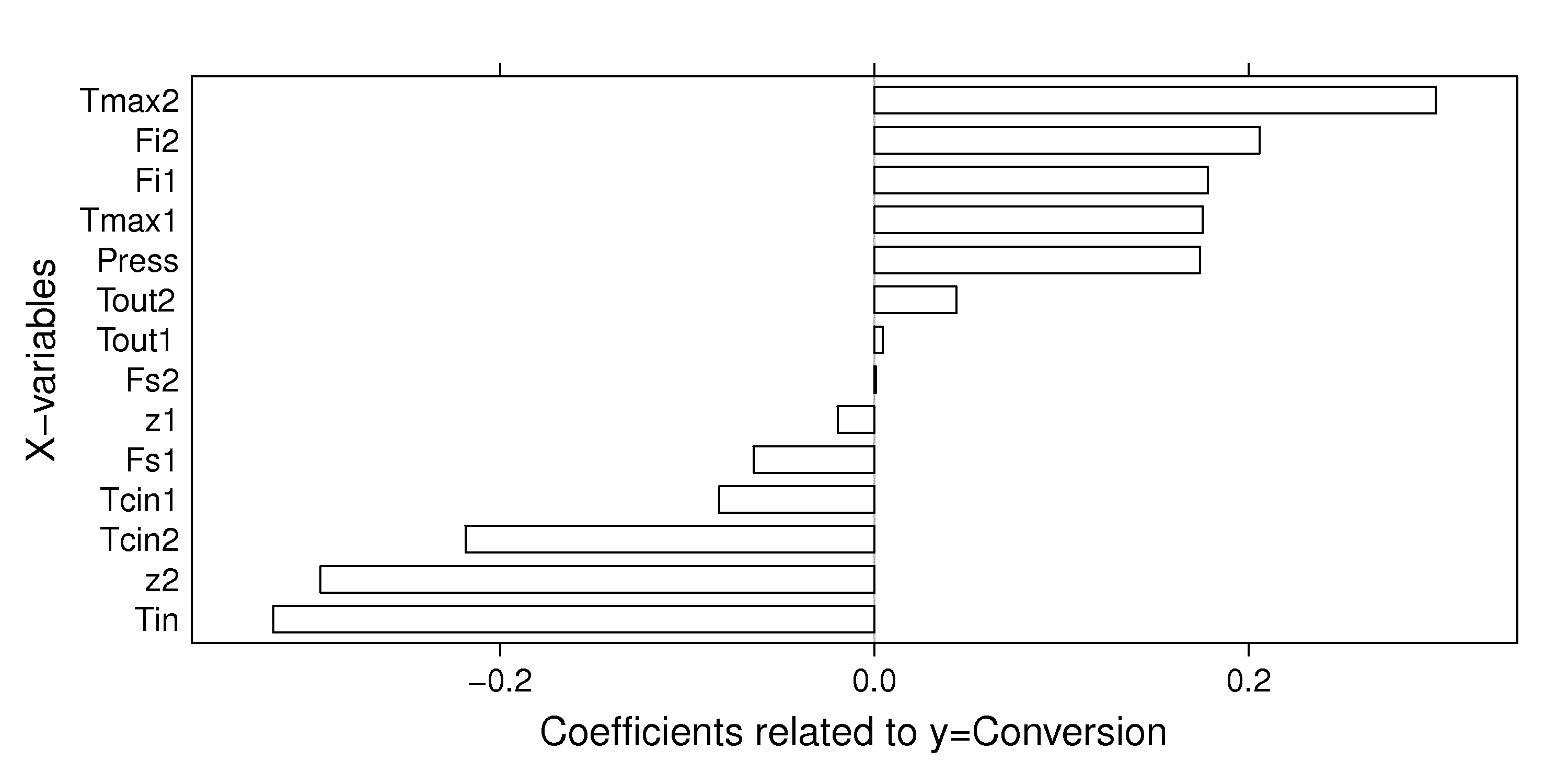
In this example the Tin, z2, Tcin2 and Tmax2, Fi2, Fi1, Tmax1, and Press variables are all related to conversion, the \(\mathrm{y}\) variable. This does not imply a cause and effect relationships, rather it just shows they are strongly correlated.