5.6. Experiments with a single variable at two levels

This is the simplest type of experiment. It involves an outcome variable, \(y\), and one input variable, \(x\). The \(x\)-variable could be a continuous numeric one, such as temperature, or discrete, such as yes/no, on/off, A/B. This type of experiment could be used to answer questions such as the following:

• Has the reaction yield increased when using catalyst A or B?

• Does the concrete’s strength improve when adding a particular binder or not?

• Does the plastic’s stretchability improve when extruded at various temperatures (a low or high temperature)?

We can perform several runs (experiments) at level A, and some runs at level B. These runs are randomized (i.e. do not perform all the A runs, and then the B runs). We strive to hold all other disturbance variables constant so we pick up only the A-to-B effect. Disturbances are any variables that might affect \(y\) but, for whatever reason, we don’t wish to quantify. If we cannot control the disturbance, then at least we can use pairing and blocking. Pairing is blocking with blocks of size two: the two runs of a pair are made under the same level of the disturbance, so its effect cancels in their difference. Blocking generalizes this to larger groups, and it is used even when there is only a single factor of interest.

5.6.1. Recap of group-to-group differences

We have already seen in the univariate statistics section how to analyze this sort of data. We first calculate a pooled variance, then a \(z\)-value, and finally a confidence interval based on this \(z\). Please refer back to that section to review the important assumptions we have to make to arrive at this equation:

\[\begin{split}s_P^2 &= \frac{(n_A -1) s_A^2 + (n_B-1)s_B^2}{n_A - 1 + n_B - 1}\\ z &= \frac{(\overline{x}_B - \overline{x}_A) - (\mu_B - \mu_A)}{\sqrt{s_P^2 \left(\frac{1}{n_A} + \frac{1}{n_B}\right)}} \\\end{split}\]

\[\begin{split}\begin{array}{rcccl} -c_t &\leq& z &\leq & c_t\\ (\overline{x}_B - \overline{x}_A) - c_t \times \sqrt{s_P^2 \left(\frac{1}{n_A} + \frac{1}{n_B}\right)} &\leq& \mu_B - \mu_A &\leq & (\overline{x}_B - \overline{x}_A) + c_t \times \sqrt{s_P^2 \left(\frac{1}{n_A} + \frac{1}{n_B}\right)} \end{array}\end{split}\]

Note

We keep the symbol \(z\) here to match the univariate section, but because the pooled variance \(s_P^2\) is estimated from the data (rather than known), this statistic is strictly \(t\)-distributed, not standard normal. That is why the critical value \(c_t\) and the degrees of freedom \(n_A + n_B - 2\) come from the \(t\)-distribution.

We consider the effect of changing from condition A to condition B to be a statistically significant effect when this confidence interval does not span zero. However, the width of this interval and how symmetrically it spans zero can cause us to come to a different, practical conclusion. In other words, we override the narrow statistical conclusion based on the richer information we can infer from the width of the confidence interval and the variance of the process.

5.6.2. How many runs at each level?

The recap above pooled the two groups into a single variance, \(s_P^2\), which already assumes the spread at level A equals the spread at level B. Before running the experiment, there is a planning question hiding inside that assumption: if the budget allows a fixed total of \(N\) runs, how many should be measured at level A and how many at level B?

Write \(n_A\) for the number of runs at level A and \(n_B = N - n_A\) for the number at level B. Keeping the two variances separate, the estimated difference \(\overline{x}_B - \overline{x}_A\) has variance

\[\text{var}\left(\overline{x}_B - \overline{x}_A\right) = \frac{\sigma_A^2}{n_A} + \frac{\sigma_B^2}{n_B}\]

where \(\sigma_A^2\) and \(\sigma_B^2\) are the variances of a single run at each level. A precise experiment makes this variance small, so the way we split the budget is itself a design choice. The function below computes the variance for every whole-run split of a budget, together with the efficiency: the smallest variance in the table divided by the variance of a given split, written as a percentage. The efficiency says how precise a split is relative to the best split of the same budget.

Python, 25 lines

import pandas as pd

def allocation_table(var_A, var_B, cost_A, cost_B, budget):
    """Variance and efficiency of every whole-run split of a fixed budget."""
    rows = []
    n_A = 1
    while cost_A * n_A < budget:
        remainder = budget - cost_A * n_A
        if remainder % cost_B == 0:
            n_B = remainder // cost_B
            variance = var_A / n_A + var_B / n_B
            rows.append((n_A, n_B, variance))
        n_A += 1
    table = pd.DataFrame(rows, columns=["n_A", "n_B", "variance"])
    table["efficiency"] = 100 * table["variance"].min() / table["variance"]
    return table

# Equal variances, equal costs, twelve runs (balanced split is best):
print(allocation_table(1, 1, 1, 1, 12))

# Level B nine times as variable as level A, equal costs, twelve runs:
print(allocation_table(1, 9, 1, 1, 12))

# Equal variances, but a run at level A costs twice as much, budget of 24:
print(allocation_table(1, 1, 2, 1, 24))

When the two levels have the same variance, \(\sigma_A^2 = \sigma_B^2 = \sigma^2\), and a run at either level costs the same, the variance is smallest when the runs are divided evenly. The first call above, with \(\sigma^2 = 1\) and \(N = 12\), gives:

Runs at A	Runs at B	Variance	Efficiency
1	11	1.091	30.6%
2	10	0.600	55.6%
3	9	0.444	75.0%
4	8	0.375	88.9%
5	7	0.343	97.2%
6	6	0.333	100.0%
7	5	0.343	97.2%
8	4	0.375	88.9%
9	3	0.444	75.0%
10	2	0.600	55.6%
11	1	1.091	30.6%

The balanced 6-and-6 split is best, matching the even division that most people would reach for. The penalty for a modest imbalance is small: a 5-and-7 split is still 97.2% efficient. The value of \(\sigma^2\) does not change any of this. Doubling it doubles every variance in the table and leaves the efficiencies, and so the best split, unchanged.

If the two levels do not have the same variance, the even split is no longer best. Suppose level B is nine times as variable as level A, so \(\sigma_A^2 = 1\) and \(\sigma_B^2 = 9\). The second call above, over the same \(N = 12\) runs, gives:

Runs at A	Runs at B	Variance	Efficiency
1	11	1.818	73.3%
2	10	1.400	95.2%
3	9	1.333	100.0%
4	8	1.375	97.0%
5	7	1.486	89.7%
6	6	1.667	80.0%
7	5	1.943	68.6%
8	4	2.375	56.1%
9	3	3.111	42.9%
10	2	4.600	29.0%
11	1	9.091	14.7%

Now the best split is 3 runs at level A and 9 at level B, and the balanced split has fallen to 80.0% efficiency. The extra runs at level B offset its larger variance, keeping the term \(\sigma_B^2 / n_B\) from dominating the sum. With equal costs the variance is smallest when the runs are shared in proportion to the standard deviations, \(n_A : n_B = \sigma_A : \sigma_B\), which places 3 and 9 runs here.

Cost can move the split away from even in the same way. Suppose the two levels have the same variance, but a run at level A costs twice as much as a run at level B, and the budget is fixed at a total cost of 24, so that \(2 n_A + n_B = 24\). The third call above finds that the variance is smallest with 7 runs at level A and 10 at level B: an unbalanced design whose total run count is not even. Combining both effects, the variance is smallest when

\[n_A : n_B = \frac{\sigma_A}{\sqrt{c_A}} : \frac{\sigma_B}{\sqrt{c_B}}\]

where \(c_A\) and \(c_B\) are the cost of a single run at each level. The general principle is to place more runs where the variance is larger and where the runs are cheaper. The even split is best only in the particular case of equal variances, equal costs, and an even number of runs. This allocation question, and the case study that motivates it, is treated in the opening chapter of Goos and Jones.

In practice the two variances are seldom known before the experiment, whereas the two costs usually are. The balanced split stayed at least 80% efficient across every case above, so it is a reasonable default when nothing is known about the variances. When a cost difference is known, the split that accounts for it can be chosen deliberately.

5.6.3. Using linear least squares models

There’s another interesting way that you can analyze data from an A versus B set of tests and get the identical result to the methods we showed in the section where we made group-to-group comparisons. In this method, instead of using a \(t\)-test, we use a least squares model of the form:

\[y_i = b_0 + g d_i\]

where \(y_i\) is the response variable \(d_i\) is an indicator variable. For example, \(d_i = 0\) when using condition A and \(d_i=1\) for condition B. Build this linear model, and then examine the confidence interval for the coefficient \(g\). The following R function uses the \(y\)-values from experiments under condition A and the values under condition B to calculate the least squares model:

S, 21 lines

lm_difference <- function(groupA, groupB)
{
    # Build a linear model with groupA = 0, and groupB = 1

    y.A <- groupA[!is.na(groupA)]
    y.B <- groupB[!is.na(groupB)]
    x.A <- numeric(length(y.A))
    x.B <- numeric(length(y.B)) + 1
    y <- c(y.A, y.B)
    x <- c(x.A, x.B)
    x <- factor(x, levels=c("0", "1"), labels=c("A", "B"))

    model <- lm(y ~ x)
    return(list(summary(model), confint(model)))
}

brittle <- read.csv('https://openmv.net/file/brittleness-index.csv')

# We developed the "group_difference" function in the Univariate section
group_difference(brittle$TK104, brittle$TK107)
lm_difference(brittle$TK104, brittle$TK107)

Use this function in the same way you did in the carbon dioxide exercise in the univariate section. For example, you will find when comparing TK104 and TK107 that \(z = 1.4056\) and the confidence interval is \(-21.4 \leq \mu_{107} - \mu_{104}\leq 119\). Similarly, when coding \(d_i = 0\) for reactor TK104 and \(d_i = 1\) for reactor TK107, we get the least squares confidence interval for parameter \(g\): \(-21.4 \leq g \leq 119\). This is a little surprising, because the first method creates a pooled variance and calculates a \(z\)-value and then a confidence interval. The least squares method builds a linear model, and then calculates the confidence interval using the model’s standard error.

Both methods give identical results, but by very different routes.

5.6.4. The importance of randomization

We emphasized in a previous section that experiments must be performed in random order to avoid any unmeasured, and uncontrolled, disturbances from impacting the system.

The concept of randomization was elegantly described in an example by Fisher in Chapter 2 of his book, The Design of Experiments. A lady claims that she can taste the difference in a cup of tea when the milk is added after the tea or when the tea is added after the milk. By setting up \(N\) cups of tea that contain either the milk first (M) or the tea first (T), the lady is asked to taste these \(N\) cups and make her assessment. Fisher shows that if the experiments are performed in random order, the actual set of decisions made by the lady are just one of many possible outcomes. He calculates all possibilities (we show how below), and then he calculates the probability of the lady’s actual set of decisions being due to chance alone. If the lady has test score values better than by random chance, then there is a reasonable claim the lady is reliable.

Let’s take a look at a more engineering-oriented example. We previously considered the brittleness of a material made in either TK104 or TK107. The same raw materials were charged to each reactor. So, in effect, we are testing the difference due to using reactor TK104 or reactor TK107. Let’s call them case A (TK104) and case B (TK107) so the notation is more general. We collected 20 brittleness values from TK104 and 23 values from TK107. We will only use the first 8 values from TK104 and the first 9 values from TK107 (you will see why soon):

Case A	254	440	501	368	697	476	188	525
Case B	338	470	558	426	733	539	240	628	517

Fisher’s insight was to create one long vector of these outcomes (length of vector = \(n_A + n_B\)) and randomly assign “A” to \(n_A\) of the values and “B” to \(n_B\) of the values. One can show that there are \(\dfrac{(n_A + n_B)!}{n_A! n_B!}\) possible combinations. For example, if \(n_A=8\) and \(n_B = 9\), then the number of unique ways to split these 17 experiments into two groups of 8 (A) and 9 (B) is 24,310 ways. For example, one way is BABB ABBA ABAB BAAB, and you would therefore assign the experimental values accordingly (B = 254, A = 440, B = 501, B = 368, A = 697, etc.).

Only one of the 24,310 sequences will correspond to the actual data printed in the above table. Although all the other realizations are possible, they are fictitious. We do this because the null hypothesis is that there is no difference between A and B. Values in the table could have come from either system.

So for each of the 24,310 realizations, we calculate the difference of the averages, \(\overline{y}_B - \overline{y}_A\), and plot a histogram of these differences. This is shown below, together with a vertical line indicating the actual realization in the table. There are 4956 permutations that had a greater difference than the one actually realized; that is, 79.6% of the other combinations had a smaller value.

Had we used a formal test of differences where we pooled the variances, we would have found a \(z\)-value of 0.8435, and the probability of obtaining that value, using the \(t\)-distribution with \(n_A + n_B - 2 = 15\) degrees of freedom, would be 79.4%. See how close they agree?

You can build the reference distribution yourself; enumerating all 24,310 splits takes under a second:

Python, 22 lines

import itertools
import numpy as np
import plotly.graph_objects as go

case_A = np.array([254, 440, 501, 368, 697, 476, 188, 525])
case_B = np.array([338, 470, 558, 426, 733, 539, 240, 628, 517])
outcomes = np.concatenate((case_A, case_B))
n_A, n_total, grand_total = len(case_A), len(outcomes), outcomes.sum()

differences = []
for subset in itertools.combinations(range(n_total), n_A):
    sum_A = outcomes[list(subset)].sum()
    differences.append((grand_total - sum_A) / (n_total - n_A) - sum_A / n_A)

observed = case_B.mean() - case_A.mean()
print(len(differences), observed, sum(d > observed for d in differences))

fig = go.Figure(go.Histogram(x=differences, nbinsx=50))
fig.add_vline(x=observed, line_color="red")
fig.update_layout(xaxis_title="Difference in averages, B minus A",
                  yaxis_title="Number of splits")
fig.show()

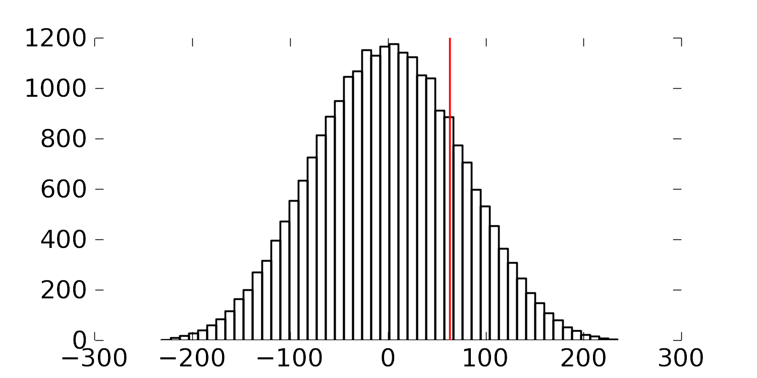
The figure shows the differences in the averages, \(\overline{y}_B - \overline{y}_A\), for the 24,310 realizations. The vertical line represents the difference in the average for the one particular set of numbers we measured in the experiment. The smooth curve is the \(t\)-distribution with 15 degrees of freedom, scaled to the same number of experiments, so that the two ways of judging the result can be compared directly.

Recall that independence is required to calculate the \(z\)-value for the average difference and compare it against the \(t\)-distribution. By randomizing our experiments, we are able to guarantee that the results we obtain from using \(t\)-distributions are appropriate. Without randomization, these \(z\)-values and confidence intervals may be misleading.

The reason we prefer using the \(t\)-distribution approach over randomization is that formulating all random combinations and then calculating all the average differences as shown here quickly becomes impractical. The complete dataset has 20 values from group A and 23 values from group B, which can be split in 960,566,918,220 ways. Enumerating them in Python takes about 3.5 seconds per million combinations on a current machine, so the full set would take around 40 days of computing, against a fraction of a second for the \(t\)-distribution result.