4.6. Least squares models with a single x-variable

The general linear least squares model is a very useful tool (in the right circumstances), and it is the workhorse for a number of algorithms in data analysis.

This part covers the relationship between two variables only: \(x\) and \(y\). In a later part on general least squares we will consider more than two variables and use matrix notation. But we start off slowly here, looking first at the details for relating two variables.

We will follow these steps:

1. Model definition (this subsection)

2. Building the model

3. Interpretation of the model parameters and model outputs (coefficients, \(R^2\), and standard error \(S_E\))

4. Consider the effect of unusual and influential data

5. Assessment of model residuals

The least squares model postulates that there is a linear relationship between measurements in vector \(x\) and vector \(y\) of the form:

(1)\[\begin{split} \mathcal{E}\left\{\mathrm{y}\right\} &= \beta_0 + \beta_1 \mathrm{x} \\ \mathrm{y} &= \beta_0 + \beta_1 \mathrm{x} + \epsilon\end{split}\]

The \(\beta_0\), \(\beta_1\) and \(\epsilon\) terms are population parameters, which are unknown (see the section on univariate statistics). The \(\epsilon\) term represents any unmodelled components of the linear model, measurement error, and is simply called the error term. Notice that the error is not due to \(x\), but is the error in fitting \(y\); we will return to this point in the section on least squares assumptions. Also, if there is no relationship between \(x\) and \(y\) then \(\beta_1 = 0\).

We develop the least squares method to estimate these parameters; these estimates are defined as \(b_0 = \hat{\beta_0}\), \(b_1 = \hat{\beta_1}\) and \(e = \hat{\epsilon}\). Using this new nomenclature we can write, for a given observation \(i\):

(2)\[\begin{split} y_i &= b_0 + b_1 x_i + e_i \\ \hat{y}_i &= b_0 + b_1 x_i\end{split}\]

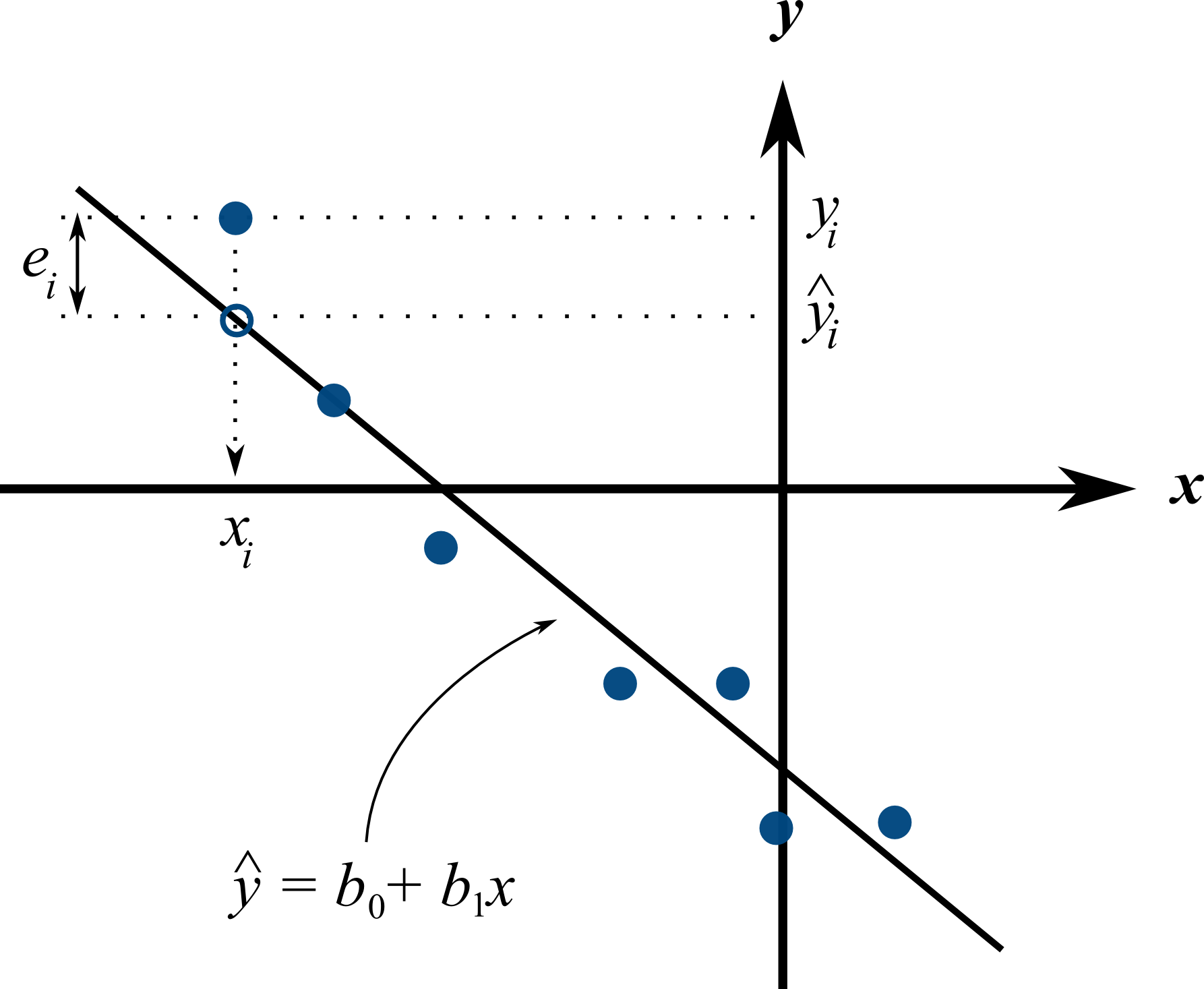
Presuming we have calculated estimates \(b_0\) and \(b_1\) we can use the model with a new x-observation, \(x_i\), and predict its corresponding \(\hat{y}_i\). The error value, \(e_i\), is generally non-zero, indicating our prediction estimate of \(\hat{y}_i\) is not exact. All this new nomenclature is illustrated in the figure.

4.6.1. Minimizing errors as an objective

Our immediate aim however is to calculate the \(b_0\) and \(b_1\) estimates from the \(n\) pairs of data collected: \((x_i, y_i)\).

Here are some valid approaches, usually called objective functions for making the \(e_i\,\) values small. One could use:

1. \(\sum_{i=1}^{n}{(e_i)^2}\), which leads to the least squares model

2. \(\sum_{i=1}^{n}{(e_i)^4}\)

3. sum of perpendicular distances to the line \(y = b_0 + b_1 x\)

4. \(\sum_{i=1}^{n}{|e_i|}\), known as the least absolute deviations model, or the \(l\)-1 norm problem

5. least median of squared error model, which is a robust form of least squares that is far less sensitive to outliers.

The traditional least squares model, the first objective function listed, has the lowest variance for \(b_0\) and \(b_1\) among all estimators that are linear in the \(y\)-values and unbiased, provided certain additional assumptions are met (this result is known as the Gauss-Markov theorem). The low variance of these parameter estimates is very desirable, for both model interpretation and using the model. The other objective functions are good alternatives and may be useful in many situations, particularly the last alternative.

Other reasons for so much focus on the least squares alternative is because it is computationally tractable by hand and very fast on computers, and it is easy to prove various mathematical properties. The other forms take much longer to calculate, almost always have to be done on a computer, may have multiple solutions, the solutions can change dramatically given small deviations in the data (unstable, high variance solutions), and the mathematical proofs are difficult. Also the interpretation of the least squares objective function is suitable in many situations: it penalizes deviations quadratically; i.e. large deviations much more than the smaller deviations.

You can read more about least squares alternatives in the book by Birkes and Dodge: “Alternative Methods of Regression”.

4.6.2. Solving the least squares problem and interpreting the model

Having settled on the least squares objective function, let’s construct the problem as an optimization problem and understand its characteristics.

The least squares problem can be posed as an unconstrained optimization problem:

(3)\[\begin{split} \min_{\displaystyle b_0, b_1} f(b_0, b_1) &= \sum_{i=1}^{n}{(e_i)^2} \\ &= \sum_{i=1}^{n}{\left(y_i - b_0 - b_1 x_i\right)^2}\end{split}\]

Returning to our example of the gas cylinder. In this case we know that \(\beta_0 = 0\) from theoretical principles. So we can solve the above problem by trial and error for \(b_1\). We expect \(b_1 \approx \beta_1 = \dfrac{nR}{V} = \dfrac{(14.1 \text{~mol})(8.314 \text{~J/(mol.K)})}{20 \times 10^{-3} \text{m}^3} = 5.861 \text{~kPa/K}\). So construct equally spaced points of \(5.0 \leq b_1 \leq 6.5\), set \(b_0 = 0\). Then calculate the objective function using the \((x_i, y_i)\) data points recorded earlier using (3).

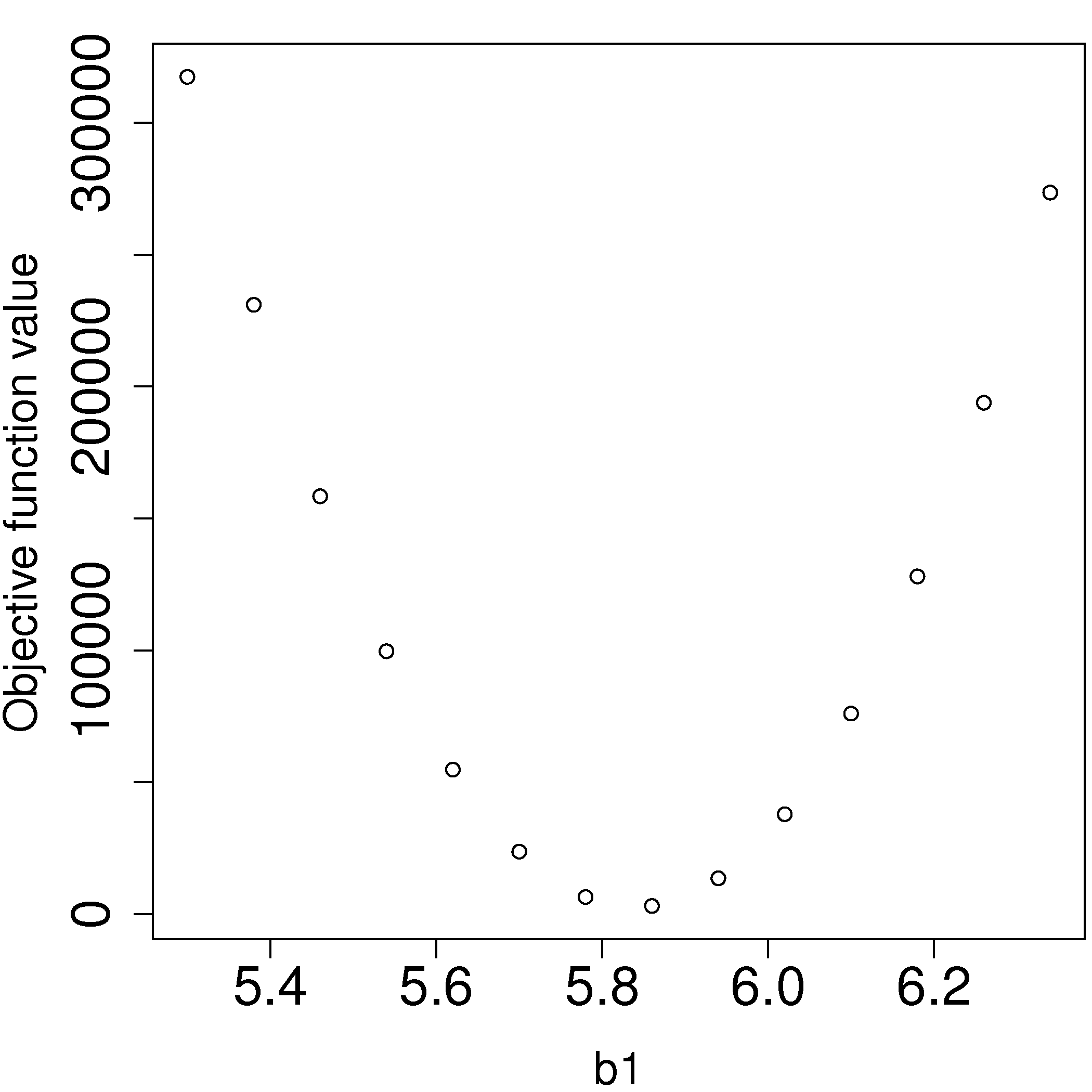
We find our best estimate for \(b_1\) roughly at 5.88, the minimum of our grid search, which is very close to the theoretically expected value of 5.86 kPa/K.

For the case where we have both \(b_0\) and \(b_1\) varying we can construct a grid and tabulate the objective function values at all points on the grid. The least squares objective function is shaped like a bowl for these cases, and a unique minimum will be found as long as there is variation in the \(x\)-data, because the objective function is convex.

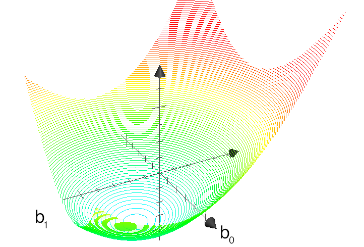
The above figure shows the general nature of the least-squares objective function where the two horizontal axes are for \(b_0\) and \(b_1\), while the vertical axis represents the least squares objective function \(f(b_0, b_1)\).

The illustration highlights the quadratic nature of the objective function. To find the minimum analytically we start with equation (3) and take partial derivatives with respect to \(b_0\) and \(b_1\), and set those equations to zero. This is a required condition at any optimal point (see a reference on optimization theory), and leads to 2 equations in 2 unknowns.

(4)\[\begin{split}\dfrac{\partial f(b_0, b_1)}{\partial{b_0}} &= -2 \sum_i^{n}{(y_i - b_0 - b_1 x_i)} = 0 \\ \dfrac{\partial f(b_0, b_1)}{\partial{b_1}} &= -2 \sum_i^{n}{(x_i)(y_i - b_0 - b_1 x_i)} = 0\\\end{split}\]

Now divide the first line through by \(n\) (the number of data pairs we are using to estimate the parameters) and solve that equation for \(b_0\). Then substitute that into the second line to solve for \(b_1\). From this we obtain the parameters that provide the least squares optimum for \(f(b_0, b_1)\):

(5)\[\begin{split}b_0 &= \overline{\mathrm{y}} - b_1\overline{\mathrm{x}} \\ b_1 &= \dfrac{ \sum_i{\left(x_i - \overline{\mathrm{x}}\right)\left(y_i - \overline{\mathrm{y}}\right) } }{ \sum_i{\left( x_i - \overline{\mathrm{x}}\right)^2} }\end{split}\]

Verify for yourself that:

1. The first part of equation (4) shows \(\sum_i{e_i} = 0\), also implying the average error is zero.

2. The first part of equation (5) shows that the straight line equation passes through the mean of the data \((\overline{\mathrm{x}}, \overline{\mathrm{y}})\) without error.

3. From second part of equation (4) prove to yourself that \(\sum_i{(x_i e_i)} = 0\), just another way of saying the dot product of the \(x\)-data and the error, \(x^Te\), is zero.

4. Also prove and interpret that \(\sum_i{(\hat{y}_i e_i)} = 0\), the dot product of the predictions and the errors is zero.

5. Notice that the parameter estimate for \(b_0\) depends on the value of \(b_1\): we say the estimates are correlated - you cannot estimate them independently.

6. You can also compute the second derivative of the objective function to confirm that the optimum is indeed a minimum.

Remarks:

1. What units does parameter estimate \(b_1\) have?

   • The units of \(y\) divided by the units of \(x\).

2. Recall the temperature and pressure example: let \(\hat{p}_i = b_0 + b_1 T_i\):

   1. What is the interpretation of coefficient \(b_1\)?

      • A one Kelvin increase in temperature is associated, on average, with an increase of \(b_1\) kPa in pressure.

   2. What is the interpretation of coefficient \(b_0\)?

      • It is the expected pressure when temperature is zero. Note: often the data used to build the model are not close to zero, so this interpretation may have no meaning.

3. What does it mean that \(\sum_i{(x_i e_i)} = x^T e = 0\) (i.e. the dot product is zero):

   • The residuals are uncorrelated with the input variables, \(x\). There is no information in the residuals that is in \(x\).

4. What does it mean that \(\sum_i{(\hat{y}_i e_i)} = \hat{y}^T e = 0\)

   • The fitted values are uncorrelated with the residuals.

5. How could the denominator term for \(b_1\) equal zero? And what would that mean?

   • This shows that as long as there is variation in the \(x\)-data that we will obtain a solution. We get no solution to the least squares objective if there is no variation in the data.

4.6.3. Example

We will refer back to the following example several times. Calculate the least squares estimates for the model \(y = b_0 + b_1 x\) from the given data. Also calculate the predicted value of \(\hat{y}_i\) when \(x_i = 5.5\)

\(x\)	10.0	8.0	13.0	9.0	11.0	14.0	6.0	4.0	12.0	7.0	5.0
\(y\)	8.04	6.95	7.58	8.81	8.33	9.96	7.24	4.26	10.84	4.82	5.68

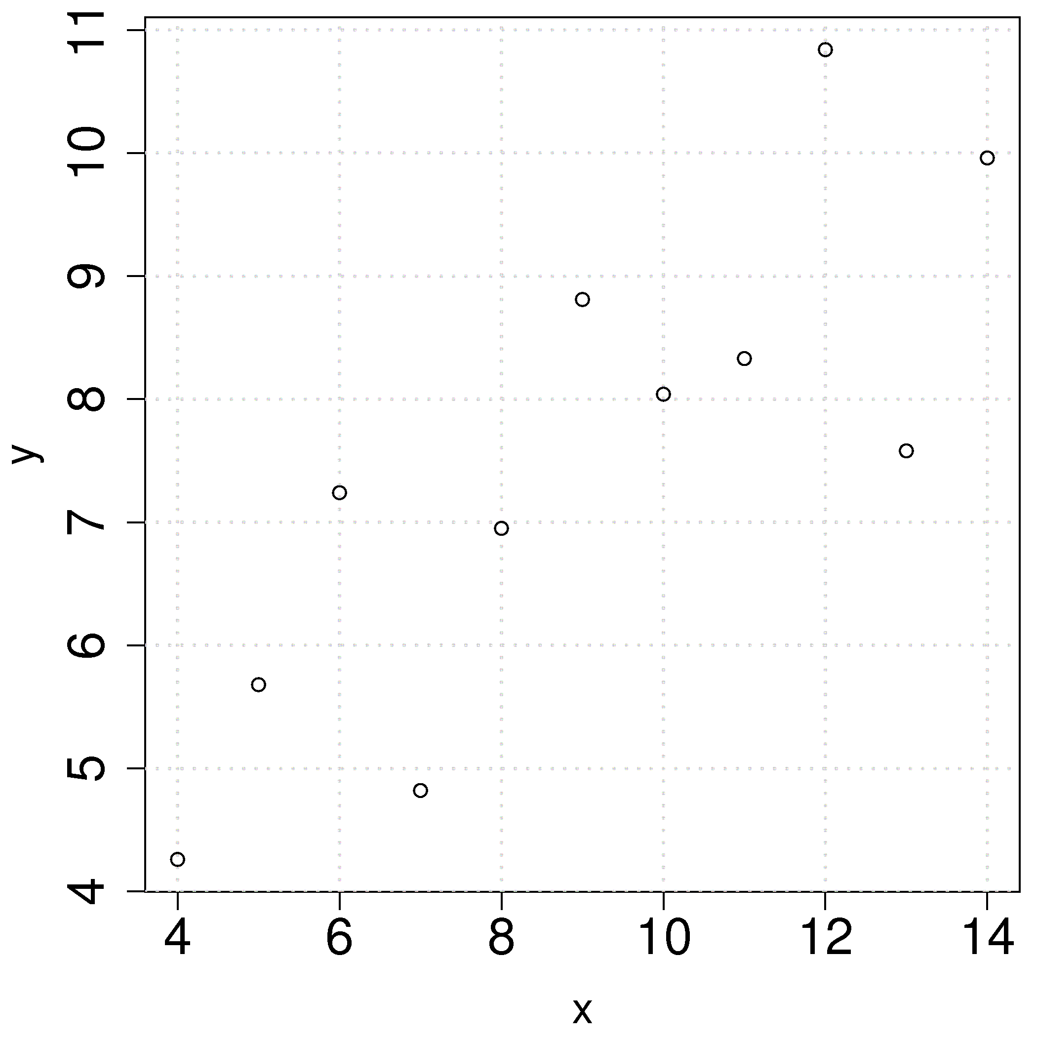
To calculate the least squares model:

Python, 31 lines

import numpy as np
import statsmodels.api as sm

x = np.array([10, 8, 13, 9, 11, 14, 6, 4, 12, 7, 5])
y = np.array([8.04, 6.95, 7.58, 8.81, 8.33, 9.96,
              7.24, 4.26, 10.84, 4.82, 5.68])

# Calculate the linear model, where y
# is described by x. add_constant adds
# the intercept term.
X = sm.add_constant(x)
mod_ls = sm.OLS(y, X).fit()

# Coefficients: the intercept first, then the
# slope. x is a NumPy array, so the entries
# are not labelled.
print(mod_ls.params)
# [3.00009091 0.50009091]

# You can get more information with
print(mod_ls.summary())

print("The model coefficients are: ")
mod_ls.params

b0, b1 = mod_ls.params
x_new = 5.5
y_predicted = b0 + b1 * x_new
print(f"Given a new x value of {x_new} "
      f"the predicted y = "
      f"{round(y_predicted, 3)}")

R, 28 lines

x <- c(10, 8, 13, 9, 11, 14, 6, 4, 12, 7, 5)
y <- c(8.04, 6.95, 7.58, 8.81, 8.33, 9.96,
      7.24, 4.26, 10.84, 4.82, 5.68)

# "Calculate for me the linear model,
# where y is described by x"
mod.ls <- lm(y ~ x)

# Call:
# lm(formula = y ~ x)
#
# Coefficients:
# (Intercept)            x
#              3.0001       0.5001

# You can get more information with
summary(mod.ls)

print('The model coefficients are: ')
coefficients(mod.ls)

b0 <- coefficients(mod.ls)[1]
b1 <- coefficients(mod.ls)[2]
x.new <- 5.5
y_predicted <- b0 + b1 * x.new
paste0('Given a new x value of ', x.new,
       ' the predicted y = ',
       round(y_predicted, 3))

• \(b_0 = 3.0\)

• \(b_1 = 0.5\)

• When \(x_i = 5.5\), then \(\hat{y}_i = 3.0 + 0.5 \times 5.5 = 5.75\)

4.6.4. A larger example: predicting vapour pressure

For larger data sets, the OLS class from the process_improve package (the Python library accompanying this book) provides a convenient API that fits naturally with Pandas data frames. It follows the scikit-learn estimator convention: the fit, predict and score methods and the intercept_ attribute work the same way in scikit-learn’s own LinearRegression class. Two details are specific to OLS: the fitted coefficients are stored in coefficients_ (scikit-learn uses coef_), and printing the fitted model gives a summary in the layout of R’s summary(lm(...)), which LinearRegression does not provide. We will use it again on the distillation tower data set introduced in the prior section.

Good statistical practice is to split the data: build the model on one part, then test it on unseen data. Otherwise we get an inflated sense of how well the model performs. The .iloc accessor in Pandas selects rows by position, so we use it to split the 253 observations into a “build” partition (the first 150 rows) and a “test” partition (the remaining rows):

Python, 11 lines

import pandas as pd

distill = pd.read_csv(
    "https://openmv.net/file/distillation-tower.csv"
)

# Use the first 150 rows to build the model,
# and the remaining rows to test it later.
build = distill.iloc[:150]
test = distill.iloc[150:]
build.shape, test.shape

Now fit a single-variable least squares model that uses InvTemp3 (the inverse of a temperature measurement on tray 3) to predict VapourPressure. The double-bracket idiom build[["InvTemp3"]] returns a column matrix (a 2-D \(n \times 1\) array). OLS.fit also accepts a 1-D array for a single predictor and reshapes it to one column itself, but the 2-D form is the one scikit-learn requires for the predictor matrix \(\mathbf{X}\), and it is the form used for the predictor matrix in the rest of this chapter:

Python, 23 lines

from process_improve.regression import OLS

# X is a 2-D array (n_rows by n_cols), the form
# scikit-learn expects. build[["InvTemp3"]] returns
# a column matrix; build["InvTemp3"] would return a
# 1-D array, which OLS.fit reshapes to one column.
X = build[["InvTemp3"]].values
y = build["VapourPressure"].values

mymodel = OLS()
mymodel.fit(X, y)

# .intercept_ is a scalar; .coefficients_ is an
# array, so we index it with [0] for the slope.
print(
    f"Intercept = {mymodel.intercept_:.5g}, "
    f"slope = {mymodel.coefficients_[0]:.5g}"
)

# Printing the model shows a summary in the same
# layout as R's summary(lm(...)), interpreted in
# the section on software output:
print(mymodel)

We will return to this model in the next section to inspect its residuals, its standard error, and its \(R^2\) value, and again in the section on multiple linear regression to extend it with a second predictor.