
 Download PDF of entire book
2.16. Exercises
Question
Recall that \(\mu = \mathcal{E}(x) = \dfrac{1}{N}\sum{x}\) and \(\mathcal{V}\left\{x\right\} = \mathcal{E}\left\{ (x - \mu )^2\right\} = \sigma^2 = \dfrac{1}{N}\sum{(x-\mu)^2}\).
What is the expected value thrown of a fair 6-sided die? (Note: plural of die is dice)
What is the expected variance of a fair 6-sided die?
Solution
Often the mean and standard deviation of a uniform distribution are not actual values from the distribution, however the definitions for them hold:
\(\mu = \mathcal{E}(x) = \dfrac{1}{N}\sum{x} = \dfrac{1}{6}(1+2+3+4+5+6) = \mathbf{3.5}\)
\(\mathcal{V}\left\{x\right\} = \mathcal{E}\left\{ (x - \mu )^2\right\} = \dfrac{1}{N}\sum{(1-3.5)^2 + (2-3.5)^2 + (3-3.5)^2 + (4-3.5)^2 + (5-3.5)^2 + (6-3.5)^2} = 17.5/6 = \mathbf{2.92}\)
If you’re feeling adventurous, you can simulate random dice rolls and verify your answers:
Code, 4 lines
> N = 10000
> hist(as.integer(runif(N, 1, 7)))      # make sure you get a uniform distribution
> mean(as.integer(runif(N, 1, 7)))      # 3.4929
> var(as.integer(runif(N, 1, 7)))       # 2.885426
Question
Characterizing a distribution: Compute the mean, median, standard deviation and MAD for salt content for the various soy sauces given in this report (page 41) as described in the the article from the Globe and Mail on 24 September 2009. Plot a box plot of the data and report the interquartile range (IQR). Comment on the 3 measures of spread you have calculated: standard deviation, MAD, and interquartile range.
The raw data are given below in units of milligrams of salt per 15 mL serving:
Code, 1 line
[460, 520, 580, 700, 760, 770, 890, 910, 920, 940, 960, 1060, 1100]
Solution
Python, 30 lines
# Salt content, mg per 15 mL serving, for 13 soy sauces.
import numpy as np
import pandas as pd
from scipy.stats import median_abs_deviation

pd.options.plotting.backend = "plotly"

salt = pd.Series([460, 520, 580, 700, 760, 770, 890, 910,
                  920, 940, 960, 1060, 1100])

print(f"mean   = {salt.mean():.1f}")          # 813.1
print(f"median = {salt.median():.0f}")        # 890
print(f"sd     = {salt.std():.1f}")           # 202.1
# scale="normal" applies the 1.4826 factor, so the MAD is comparable
# with the standard deviation for normally distributed data.
print(f"MAD    = {median_abs_deviation(salt, scale='normal'):.1f}")   # 192.7
q1, q3 = np.percentile(salt, [25, 75])
print(f"IQR    = {q3 - q1:.0f}")              # 240 = 940 - 700

fig = salt.plot.box()
fig.update_layout(yaxis_title_text="Salt content (mg / 15mL serving)",
                  showlegend=False)
fig.show()

# Testing robustness: replace one value with an artificial outlier.
salt[1] = 91941
print(f"mean   = {salt.mean():.0f}")          # 7845, not robust at all
print(f"median = {salt.median():.0f}")        # 910, robust
print(f"sd     = {salt.std():.0f}")           # 25268, way off
print(f"MAD    = {median_abs_deviation(salt, scale='normal'):.1f}")   # 222.4
or the equivalent in R:
S, 22 lines
salt <- c(460, 520, 580, 700, 760, 770, 890, 910, 920, 940, 960, 1060, 1100)
mean(salt)                                  # 813.077
median(salt)                                # 890
sd(salt)                                    # 202.0885
mad(salt)                                   # 192.738
1.4826*median(abs(salt - median(salt)))     # 192.738
IQR(salt)                                   # 240 = 940 - 700 (see below)
summary(salt)
#   Min. 1st Qu.  Median    Mean 3rd Qu.    Max.
# 460.0   700.0   890.0   813.1   940.0  1100.0

boxplot(salt, ylab="Salt content (mg / 15mL serving)")

# Testing robustness.  Create an artificial outlier
# ------------------
salt[2] = 91941
mean(salt)                                  # 7845.462   <---- not robust at all
median(salt)                                # 910        <---- robust
sd(salt)                                    # 25268.22   <---- way off!
mad(salt)                                   # 222.39     <---- robust
1.4826*median(abs(salt - median(salt)))     # 222.39     <---- manual calculation of MAD
IQR(salt)                                   # 200        <---- robust

Note that the units of spread are the same as the variable being quantified. The IQR is 240 mg salt/15 mL serving. The standard deviation (202 mg salt/15 mL serving), and MAD (193 mg salt/15 mL serving), are 2 other ways to quantify the spread of the data. Note that the IQR, for normally distributed data, will only be consistent if you divide the result by 1.349. Read the help for the IQR function in R for more details. Note from the code how the IQR is a distance between two points.
In this example the numbers are mostly in agreement, because there are no major outliers. The MAD and IQR are two robust methods of quantifying spread, while the standard deviation is extremely sensitive to outliers - due to the squaring of residuals about the mean. You can verify this by replacing one of the values and recalculating the numbers.
Question
Give a reason why Statistics Canada reports the median income when reporting income by geographic area. Where would you expect the mean to lie, relative to the median? Use this table to look up the income for Hamilton. How does it compare to Toronto? And all of Canada?
Solution
We described how easily the mean is influenced by unusual data points. Take any group of people anywhere in the world, and there will always be a few who earn lots of money (not everyone can be the CEO, especially of a bank!). Also, since no one earns negative income, the distribution piles up at the left, with fewer people on the right. This implies that the mean will lie above the median, since 50% of the histogram area must lie below the median, by definition. A previous student pointed out that low income earners are less likely to file tax returns, so they are underrepresented in the data.
Even though the median is a more fair way of reporting income, and robust to unusual earners (many low income earners, very few super-rich), I would prefer if Statistics Canada released a histogram - that would tell a lot more - even just the MAD, or IQR would be informative. It was surprising that Hamilton showed higher median earnings per family than Toronto. I infer from this that there are more low income earners in Toronto and Canada than in Hamilton, but without the histograms it is hard to be sure. Also, I wasn’t able to find exactly what StatsCan means by a family - did they include single people as a “family”? Maybe there are more, wealthy singles in Toronto, but they are aren’t included in the numbers. The median income per person would be a useful statistic to help judge that.
Question
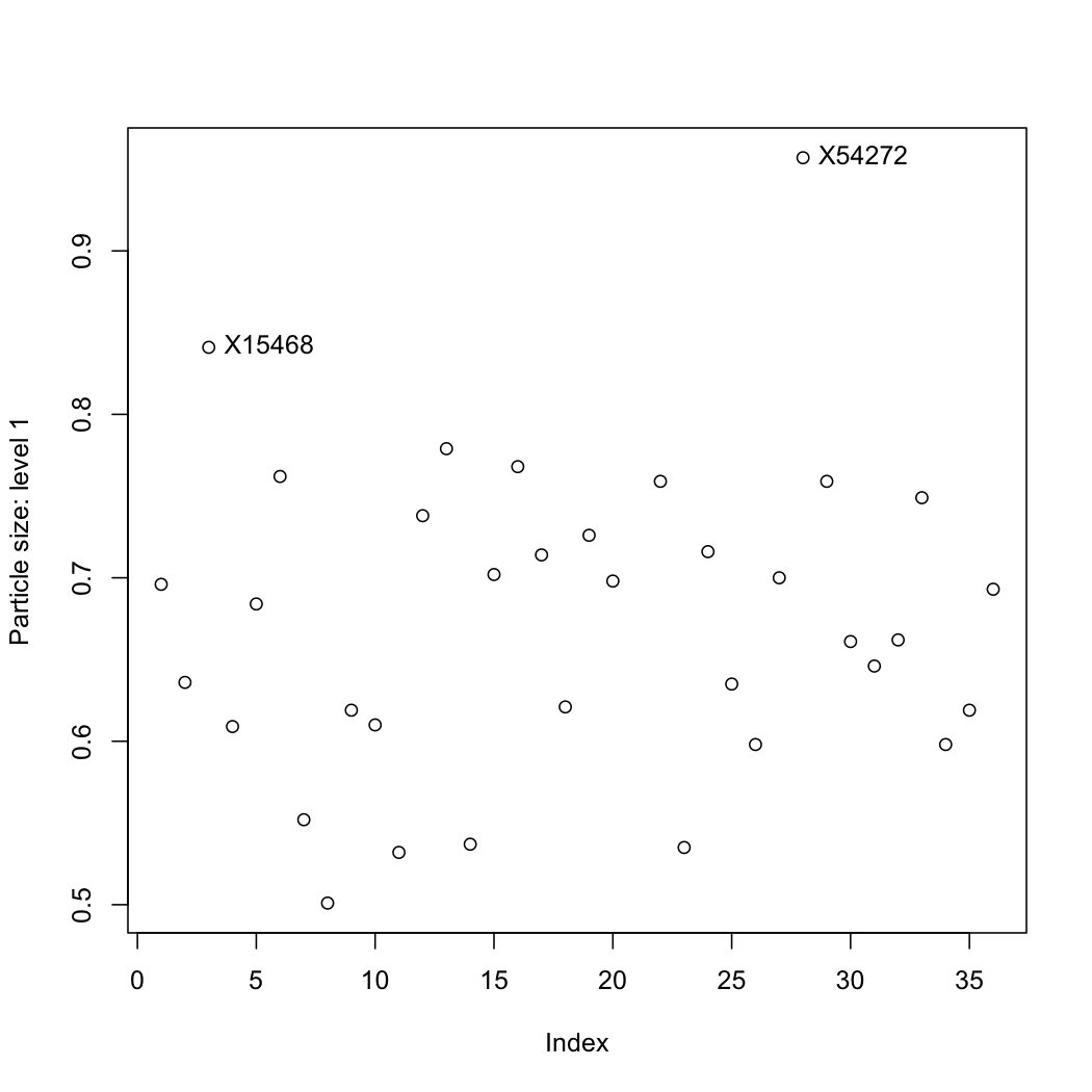
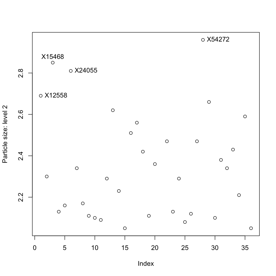
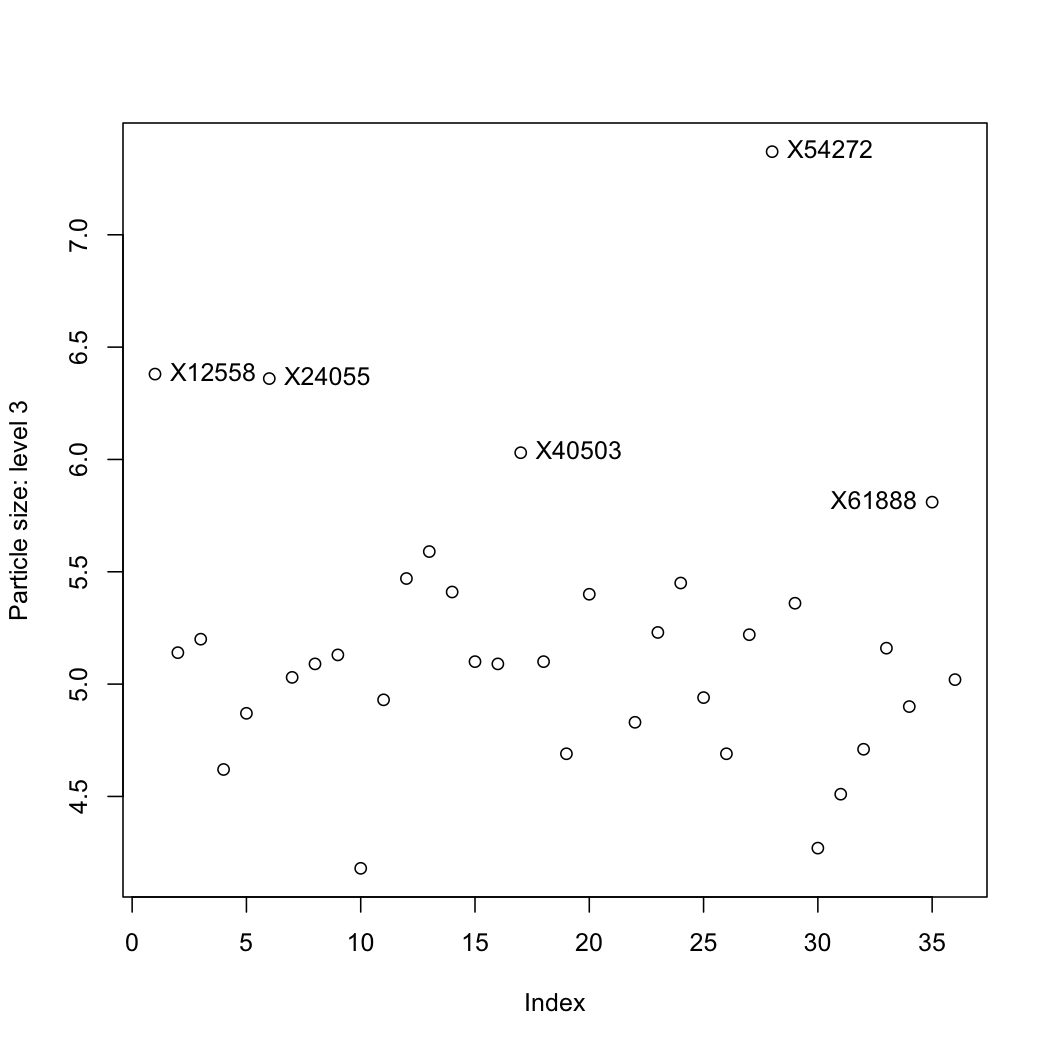
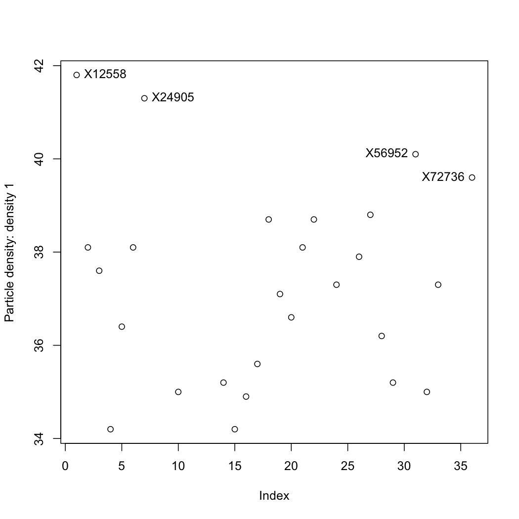
Use the data set on raw materials.
How many variables in the data set?
How many observations?
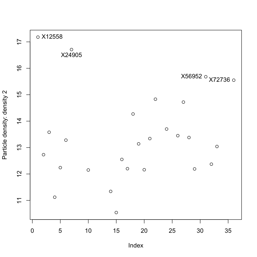
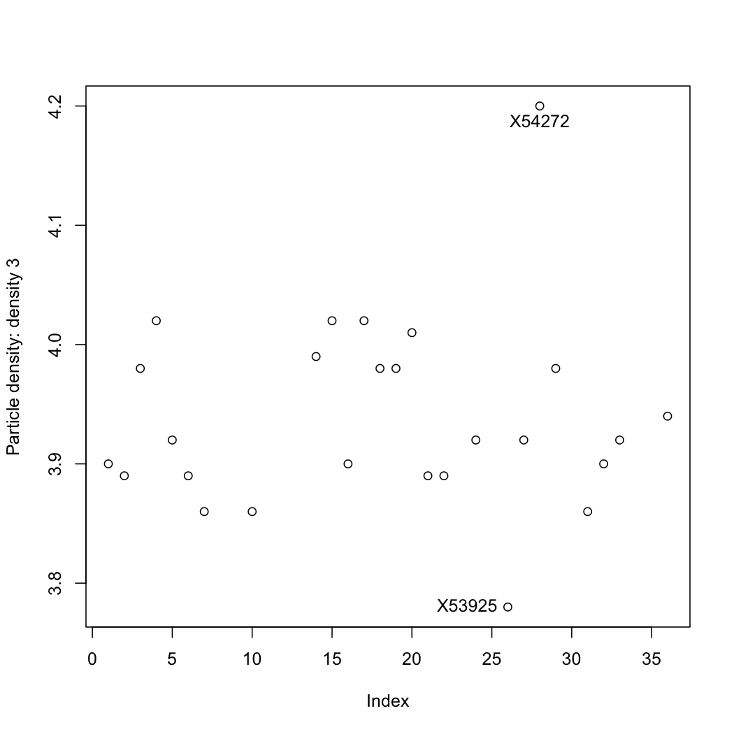
The data are properties of a powder. Plot each variable, one at a time, and locate any outliers. R-users will benefit from the R tutorial (see the use of the
identifyfunction).
Solution
See the code below that generates the plots. Outliers were identified by visual inspection of these plots. Recall an outlier is an unusual/interesting point, and a function of the surrounding data. You can use a box plot to locate preliminary outliers, but recognize that you are leaving the computer to determine what is unusual. Automated outlier detection systems work moderately well, but there is no substitute (yet!) for visual inspection of the data.
The same few samples appear to be outliers in most of the variables.
Python, 31 lines
# Properties of a powder: plot each variable in sequence order and
# look for unusual points.
import numpy as np
import pandas as pd

pd.options.plotting.backend = "plotly"

raw = pd.read_csv("https://openmv.net/file/raw-material-properties.csv")
print(raw.shape)     # (36, 7): 36 observations of 7 columns

labels = {
    "size1": "Particle size: level 1",
    "size2": "Particle size: level 2",
    "size3": "Particle size: level 3",
    "density1": "Particle density: level 1",
    "density2": "Particle density: level 2",
    "density3": "Particle density: level 3",
}
for column, label in labels.items():
    fig = raw[column].plot.line(markers=True, text=raw["Sample"])
    fig.update_traces(mode="markers", hovertemplate="%{text}: %{y}")
    fig.update_layout(xaxis_title_text="Index",
                      yaxis_title_text=label,
                      showlegend=False)
    fig.show()

    # Which samples fall outside the 1.5 IQR fences?
    q1, q3 = np.percentile(raw[column].dropna(), [25, 75])
    iqr = q3 - q1
    beyond = (raw[column] < q1 - 1.5 * iqr) | (raw[column] > q3 + 1.5 * iqr)
    print(column, list(raw.loc[beyond, "Sample"]))
or the equivalent in R, where identify() lets you click on the
interesting points:
S, 27 lines
rm <- read.csv('http://openmv.net/file/raw-material-properties.csv')

ncol(rm)    # 7 columns
nrow(rm)    # 36 rows

# Plot the data as you normally would
plot(rm$size1, ylab="Particle size: level 1")

# Now use the identify(...) command, with the same data as you plotted. Use the
# "labels" option to let R use the "Sample" column to label points where you click
identify(rm$size1, labels=rm$Sample)

# After issuing the "identify(...)" command, click on any interesting points in the
# plot.  Right-click anywhere to stop selecting points.


# Repeat with the other columns
plot(rm$size2, ylab="Particle size: level 2")
identify(rm$size2, labels=rm$Sample)
plot(rm$size3, ylab="Particle size: level 3")
identify(rm$size3, labels=rm$Sample)
plot(rm$density1, ylab="Particle density: level 1")
identify(rm$density1, labels=rm$Sample)
plot(rm$density2, ylab="Particle density: level 2")
identify(rm$density2, labels=rm$Sample)
plot(rm$density3, ylab="Particle density: level 3")
identify(rm$density3, labels=rm$Sample)
Question
Write a few notes on the purpose of feedback control, and its effect on variability of process quality.
Solution
Purpose is to keep the process close to a desired set point (or mean).
Sometimes used to maintain the process variability within a desired tolerance limit (or standard deviation).
Lowers the variability of the process outputs (i.e., narrow the distribution) by actually introducing greater variability into the process, to counteract external variation in the the process inputs. For example, variation from the raw materials, or ambient conditions, such as seasonal temperature are process inputs.
Feedback control allows us to move the process operation closer to targets, without less likelihood of deviation outside these limits. (In the next section on process monitoring we will learn how to track and quantify this).
Question
Use the section on Historical data from Environment Canada’s website and use the Customized Search option to obtain data for the HAMILTON A station from 2000 to 2009. Use the settings as Year=2000, and Data interval=Monthly and request the data for 2000, then click Next year to go to 2001 and so on.
For each year from 2000 to 2008, get the total snowfall and the average of the
Mean tempover the whole year (the sums and averages are reported at the bottom of the table).Plot these 2 variables against time
Now retrieve the long-term averages for these data from a different section of their website (use the same location,
HAMILTON A, and check that the data range is 1971 to 2000). Superimpose the long-term average as a horizontal line on your previous plot.Note: the purpose of this exercise is more for you to become comfortable with web-based data retrieval, which is common in most companies.
Note: please use any other city for this question if you prefer.
Solution
These are the data, and the code to plot the results. The temperature for the last decade trended higher than the average for the prior 3 decades, 1971 to 2000.
Python, 22 lines
# HAMILTON A: total annual snowfall and the average of the monthly
# mean temperature, 2000 to 2008, against the 1971 to 2000 normals.
import pandas as pd
import plotly.graph_objects as go

weather = pd.DataFrame({
    "Year": range(2000, 2009),
    "Snowfall": [170.9, 94.1, 138.0, 166.2, 175.8, 218.4, 56.6, 182.4, 243.2],
    "Temperature": [7.6, 8.8, 8.8, 7.3, 7.7, 8.2, 9.1, 8.2, 7.7],
})
normals = {"Snowfall": 161.8, "Temperature": 7.6}
titles = {"Snowfall": "Snowfall (cm)",
          "Temperature": "Average annual temperature (°C)"}

for column, title in titles.items():
    fig = go.Figure()
    fig.add_scatter(x=weather["Year"], y=weather[column], mode="lines+markers")
    fig.add_hline(y=normals[column], line_dash="dash",
                  annotation_text="Averaged over 1971 to 2000 data")
    fig.update_layout(xaxis_title_text="Year", yaxis_title_text=title,
                      showlegend=False)
    fig.show()
or the equivalent in R:
S, 14 lines
snow <- c(170.9, 94.1, 138.0, 166.2, 175.8, 218.4, 56.6, 182.4, 243.2)
temp <- c(7.6,   8.8,  8.8,   7.3,   7.7,   8.2,   9.1 , 8.2,  7.7)
year <- seq(2000, 2008)

snow.long.average = 161.8
temp.long.average = 7.6

plot(year, snow, xlab="Year", ylab="Snowfall (cm)", type="b")
abline(h=snow.long.average, col = "gray40")
text(2006, snow.long.average-5, "Total annual snowfall, averaged over 1971 to 2000 data")

plot(year, temp, xlab="Year", ylab="Average annual temperature (°C)", type="b")
abline(h=temp.long.average, col = "gray40")
text(2006, temp.long.average-0.1, "Average annual temperature, averaged over 1971 to 2000 data")


Question
Does the number of visits in the website traffic data set follow a normal distribution? If so, what are the parameters for the distribution? What is the likelihood that you will have between 10 and 30 visits to the website?
Solution
Python, 27 lines
# Do the daily website visits follow a normal distribution?
import numpy as np
import pandas as pd
from scipy import stats

pd.options.plotting.backend = "plotly"

web = pd.read_csv("https://openmv.net/file/website-traffic.csv")
visits = web["Visits"]

fig = visits.plot.hist()
fig.update_layout(xaxis_title_text="Number of visits", showlegend=False)
fig.show()

# A q-q plot: sorted data against the matching normal quantiles.
ordered = np.sort(visits)
quantiles = stats.norm.ppf((np.arange(1, len(ordered) + 1) - 0.375)
                           / (len(ordered) + 0.25))
fig = pd.DataFrame({"Normal quantiles": quantiles,
                    "Visits": ordered}).plot.scatter(x="Normal quantiles",
                                                    y="Visits")
fig.show()

mean, sd = visits.mean(), visits.std()
print(f"mean = {mean:.2f}, sd = {sd:.2f}")            # 22.23 and 8.33
inside = stats.norm.cdf((30 - mean) / sd) - stats.norm.cdf((10 - mean) / sd)
print(f"P(10 < visits < 30) = {inside:.3f}")          # 0.753
or the equivalent in R:
S, 19 lines
web <- read.csv('http://openmv.net/file/website-traffic.csv')
summary(web)

# Check for normality: use a qq-plot
qqnorm(web$Visits)
qqline(web$Visits)

# Use the qq.plot function from the "car" package for qq-plots with error bars
library(car)
qq.plot(web$Visits)

# Mean and standard deviation
visits.mean <- mean(web$Visits)              # 22.23364
visits.sd <- sd(web$Visits)                  #  8.331826

z.LB <- (10 - visits.mean) / visits.sd
z.UB <- (30 - visits.mean) / visits.sd
c(z.LB, z.UB)                                # -1.4683029  0.9321312
pnorm(z.UB) - pnorm(z.LB)                    #  0.7533546
The above source code was used to generate these plots to answer the question. The data do appear to follow a normal distribution. This means we can calculate the mean and standard deviation from the data.
Mean number of visits = 22 visits
Standard deviation of the number of visits = 8.3 visits
Probability that there are between 10 and 30 visits to the site each day: 75.3%
We should use the \(t\)-distribution to answer the last part, but at this stage we had not yet looked at the \(t\)-distribution. However, the large number of observations (214) means the \(t\)-distribution is no different than the normal distribution.
Question
The ammonia concentration in your wastewater treatment plant is measured every 6 hours. The data for one year are available from the dataset website.
Use a visualization plot to hypothesize from which distribution the data might come. Which distribution do you think is most likely? Once you’ve decided on a distribution, use a qq-plot to test your decision.
Estimate location and spread statistics assuming the data are from a normal distribution. You can investigate using the
fitdistrfunction in R, in the MASS package.What if you were told the measured values are not independent. How does it affect your answer?
What is the probability of having an ammonia concentration greater than 40 mg/L when:
you may use only the data (do not use any estimated statistics)
you use the estimated statistics for the distribution?
Note: Answer this entire question using computer software to calculate values from the normal distribution. But also make sure you can answer the last part of the question by hand, (when given the mean and variance), and using a table of normal distributions.
Solution
S, 43 lines
nh4 <- read.csv('http://openmv.net/file/ammonia.csv')
summary(nh4$Ammonia)              # just to check if the data seem OK
#    Min. 1st Qu.  Median    Mean 3rd Qu.    Max.
#    9.99   30.22   36.18   36.09   42.37   58.74

# Investigate the histogram or density plots first
hist(nh4$Ammonia)
plot(density(nh4$Ammonia))

# The qq-plot confirms it is normal, apart from the right-hand-side tail
library(car)
png(file='ammonia-qqplot.png')
qqPlot(nh4$Ammonia)
dev.off()

# Estimate the parameters of the distribution
nh4.mean = mean(nh4$Ammonia)  # 36.09499
nh4.sd = sd(nh4$Ammonia)      # 8.518928

# Advanced: use the MASS package in R to estimate
# (very similar results)
fitdistr(nh4$Ammonia, "normal")


level <- 40

# Using only the data to calculate p(Ammonia > level):
# calculate fraction of samples greater than ``level``
sum(nh4$Ammonia > level) / length(nh4$Ammonia)

# Using the normal distribution to estimate p(Ammonia > level):

# Calculate a z-value first, then the cumulative probability
z <- (level - nh4.mean)/nh4.sd
1 - pnorm(z)

# Or, you can get the answer more directly:
1 - pnorm(level, mean=nh4.mean, sd=nh4.sd)

# More correctly, we should have used the t-distribution,
# because we actually estimated the standard deviation
# We basically get the same answer
1 - pt(z, df=(length(nh4$Ammonia)-1))
When plotting a histogram, it seems that an appropriate distribution might be the normal distribution. A qq-plot shows it it mostly normal, apart from the right hand side tail (upper tail) which is slightly heavier, outside the given limits, than would be found on the normal distribution.
Assuming the data are normal, we can calculate the distribution’s parameters as \(\overline{x} = \hat{\mu} = 36.1\) and \(s= \hat{\sigma} = 8.52\).
The fact that the data are not independent is not an issue. To calculate estimates of the parameter’s distribution (the mean and standard deviation) we do not need to assume independence. One way to see this: if I randomly reorder the data, I will still get the same value for the mean and standard deviation. The assumption of independence is required for the central limit theorem, but we have not used that theorem here.
The probability of having an ammonia concentration greater than 40 mg/L:
When counting the fraction of the samples greater than 40 mg/L (i.e. we only use the data themselves): 3.44% (see code)
When using the estimated values of the mean and standard deviation from the normal distribution, we can calculate a \(z\)-value, then find the area under the normal distribution corresponding to this \(z\): 3.23% (see code)
Note: We should use actually be using the \(t\)-distribution, since we used an estimate of the population variance and not the true population variance to calculate \(z\). However, since the degrees of freedom, \(n-1 = 1439\), are so large, there is no practical difference in our answer.
Question
We take a large bale of polymer composite from our production line and using good sampling techniques, we take 9 samples from the bale and measure the viscosity in the lab for each sample. These samples are independent estimates of the population (bale) viscosity. We will believe these samples follow a normal distribution (we could confirm this in practice by running tests and verifying that samples from any bale are normally distributed). Here are 9 sampled values: 23, 19, 17, 18, 24, 26, 21, 14, 18.
The sample average
An estimate of the standard deviation
What is the distribution of the sample average, \(\overline{x}\)? What are the parameters of that distribution?
Additional information: I use a group of samples and calculate the mean, \(\overline{x}\), then I take another group of samples and calculate another \(\overline{x}\), and so on. Those values of \(\overline{x}\) are not going to be the same, but they should be similar. In other words, the \(\overline{x}\) also has a distribution. So this question asks what that distribution is, and what its parameters are.
Construct an interval, symbolically, that will contain, with 95% certainty (probability), the population mean of the viscosity.
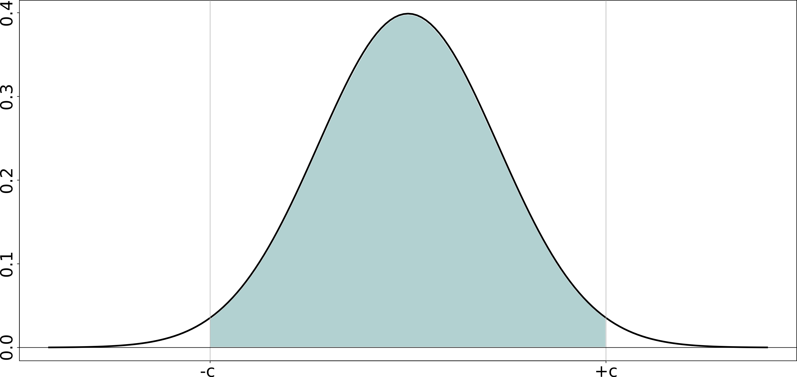
Additional information: To answer this part, you should move everything to \(z\)-coordinates first. Then you need to find the points \(-c\) and \(+c\) in the following diagram that mark the boundary for a 95% of the total area under the distribution. This region is an interval that will contain, with 95% certainty, the population mean of the viscosity, \(\mu\). Write your answer in form: \(\text{LB} < \mu < \text{UB}\).
Now assume that for some hypothetical reason we know the standard deviation of the bale’s viscosity is \(\sigma=3.5\) units, calculate the population mean’s interval numerically.
Additional information: In this part you are just finding the values of \(\text{LB}\) and \(\text{UB}\)
Solution
S, 13 lines
data <- c(23, 19, 17, 18, 24, 26, 21, 14, 18)
N = length(data)

# Mean and standard deviation
data.mean <- mean(data)
data.sd <- sd(data)
cn <- qnorm(1 - 0.05/2)

# Assume we know sigma:
sigma <- 3.5
LB <- data.mean - cn * sigma / sqrt(N)
UB <- data.mean + cn * sigma / sqrt(N)
c(LB, UB)
Sample average = 20
Sample standard deviation = 3.81
By the central limit theorem, and if the samples are taken independently, the mean, \(\overline{x} \sim \mathcal{N}\left(\mu, \sigma/\sqrt{n}\right)\)
The z-value for \(\overline{x}\) can be constructed as \(z = \dfrac{\overline{x} - \mu}{\sigma/\sqrt{n}}\). An interval within which we can find \(\mu\) with 95% certainty is given below where \(c_n\) is found from the normal distribution, and in R:
qnorm(0.975) = 1.959964, approximately 1.96.
The 95% confidence interval for \(\mu\) is from 17.7 to 22.3.
Question
You are responsible for the quality of maple syrup produced at your plant. Historical data show that the standard deviation of the syrup viscosity is 40 cP. How many lab samples of syrup must you measure so that an estimate of the syrup’s long-term average viscosity is inside a range of 60 cP, 95% of the time? This question is like the previous one: except this time you are given the range of the interval \(\text{UB}\,-\,\text{LB}\), and you need to find \(n\).
Solution
We can write the range symbolically as:
Subtracting and setting equal to 60 cP:
Question
Your manager is asking for the average viscosity of a product that you produce in a batch process. Recorded below are the 12 most recent values, taken from consecutive batches. State any assumptions, and clearly show the calculations which are required to estimate a 95% confidence interval for the mean. Interpret that confidence interval for your manager, who is not sure what a confidence interval is.
Ensure you can also complete the question by hand, using statistical tables.
Solution
The confidence interval for a mean requires the assumption that the individual numbers are taken from a normal distribution, and they are sampled independently (no sample has an effect on the others). Under these assumptions we can calculate a \(z\)-value for the sampled mean, \(\overline{x}\), and construct upper and lower bounds reflecting the probability of sampling that \(z\)-value.
Since we don’t know the value of \(\sigma\), we use the sampled value, \(s=1.16\). But this means our \(z\)-value is no longer normally distributed, rather it is \(t\)-distributed. The limits, \(\pm c_t\) that contain 95% of the area under the \(t\)-distribution, with 11 degrees of freedom, are 2.20 (or any close approximation from the tables provided). From this we get the confidence interval:
This confidence interval means that we have 95% confidence that the true average viscosity lies within these bounds. If we took 100 groups of 12 samples, then the limits calculated from 95 of those groups are expected to contain the true mean. It is incorrect to say that there is 95% probability the true mean lies within these bounds; the true mean is fixed, there is no probability associated with it.
Question
A new wastewater treatment plant is being commissioned and part of the commissioning report requires a statement of the confidence interval of the biochemical oxygen demand (BOD). How many samples must you send to the lab to be sure the true BOD is within a range of 2 mg/L, centered about the sample average? If there isn’t enough information given here, specify your own numbers and assumptions and work with them to answer the question.
Solution
The objective is to calculate \(n\), the number of samples. Let \(\overline{x}\) be the average of these \(n\) samples, and this average will be distributed according to the normal distribution with mean and standard deviation as shown below, if the samples are taken independently (which may not be possible in practice!):
The value of \(z\) will lie within this confidence interval:
At this point all we know is that UB - LB = 2 mg/L. These are the rest of the assumptions we have to make:
assume a standard deviation of \(\hat{\sigma}_{\text{BOD}}\) = 4 mg/L
use 95% confidence intervals
assume we know the population standard deviation, so we use the normal distribution to calculate \(c_n\) as
qnorm(1-0.05/2)in R.
Solving for \(n\) at these values gives: \(n = \left(\dfrac{2(1.96)(\hat{\sigma}_{\text{BOD}})}{2}\right)^2 = (1.96 \times 4)^2 \sim 62\). This large number of samples makes sense: compare the range (2 mg/L) to the standard deviation of 4 mg/L: you have to take a large number of samples to get your precision up when you have so much noise in your signal.
Question
One of the questions we posed at the start of this chapter was: Here are the yields from a batch bioreactor system for the last 3 years (300 data points; we run a new batch about every 3 to 4 days).
What sort of distribution do the yield data have?
A recorded yield value was less than 60%, what are the chances of that occurring? Express your answer as: there’s a 1 in n chance of it occurring.
Which assumptions do you have to make for the second part of this question?
Solution
Assume the 300 data points represent an entire population. Plot a
qqPlot(...)using thecarpackage:
The data appear to follow a normal distribution, based on the visual test of this qq-plot.
We need to find the probability that the yield, \(Y\), is less than or equal to 60, stated as \(P(Y\le 60)\). If we assume \(Y \sim \mathcal{N}(\mu,\sigma^{2})\) then we first need to find the \(z\)-value bound corresponding to 60, and then find the probability of finding values below, or equal to that bound.
\[z_\text{bound} = \frac{y-\mu}{\sigma} = \frac{60-80.353}{6.597} = -3.085\]In this data set of 300 numbers there are zero entries below this limit. But using the distribution’s fit, we can calculate the probability as
pnorm(-3.085), which is \(\approx 0.001\). This is equivalent to saying that there is a 1 in 1000 chance of achieving a yield less than 60%.We only had to assume the data are normally distributed - we did not need the data to be independent - in order to use the estimated parameters from the distribution to calculate the probability.
S, 19 lines
# import data
data <- read.csv('http://openmv.net/file/batch-yields.csv')

# Determine statistics
summary(data)
yield <- data$Yield
yield.mean <- mean(yield)
yield.sd <- sd(yield)


# Rather use a qqplot with limits
library(car)
png(file='ammonia-qqplot.png')
qqPlot(yield)
dev.off()

# Assuming normal distribution determine probability of x < 60
z <- (60-yield.mean)/yield.sd
p <- pnorm(z,0,1)
Question
One aspect of your job responsibility is to reduce energy consumption on the plant floor. You ask the electrical supplier for the energy requirements (W.h) for running a particular light fixture for 24 hours. They won’t give you the raw data, only their histogram when they tested randomly selected bulbs (see the data and code below).
S, 4 lines
> bin.centers <- c(4025, 4075, 4125, 4175, 4225, 4275, 4325, 4375)
> bin.counts <- c(4, 19, 14,  5,  4,  1,  2,  1)
> barplot(bin.counts, names.arg=bin.centers, ylab="Number of bulbs (N=50)",
     xlab="Energy required over 24 hours (W.h)", col="White", ylim=c(0,20))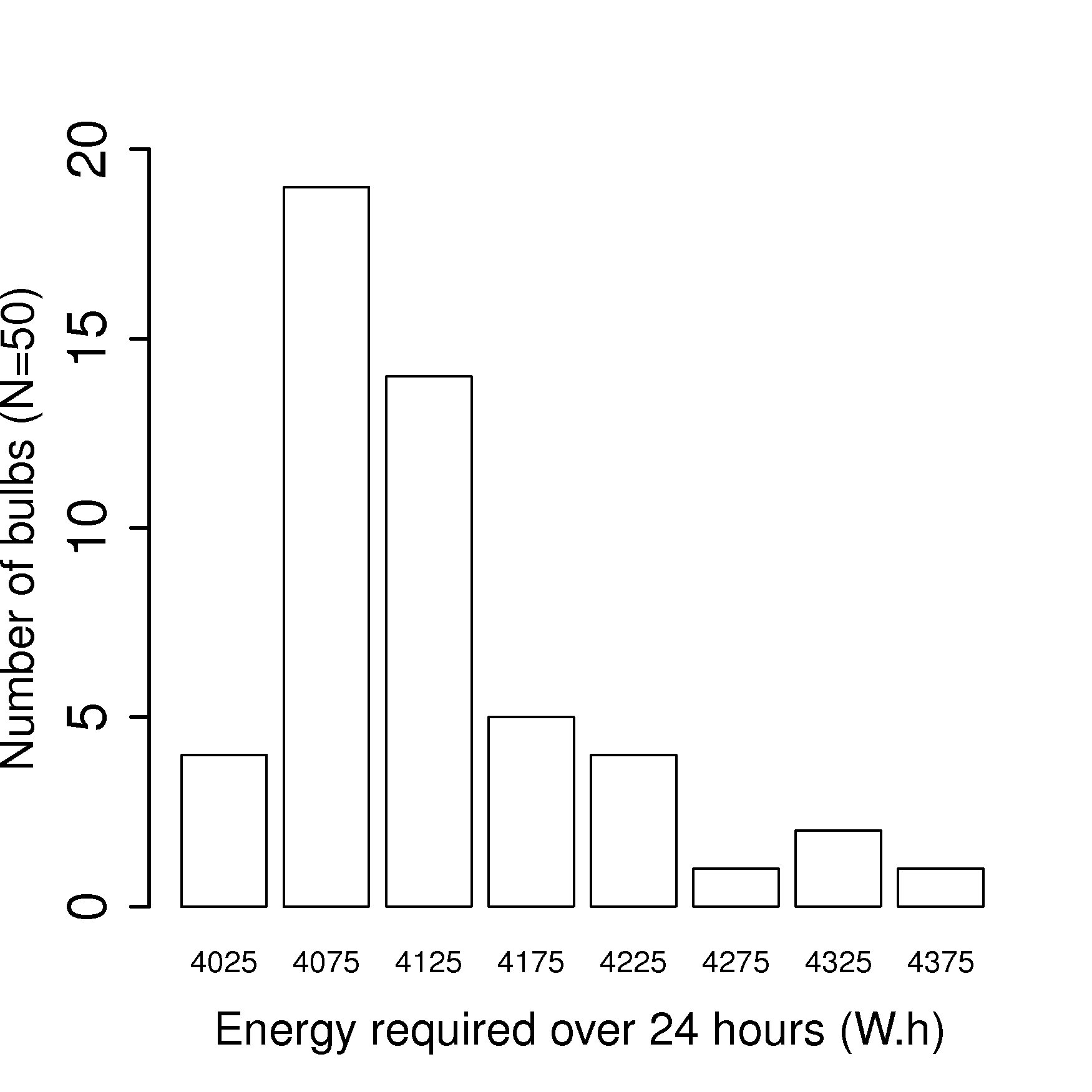
Calculate an estimate of the mean and standard deviation, even though you don’t have the original data.
What is a confidence interval for the mean at 95% probability, stating and testing any assumptions you need to make.
Solution
The mean and standard deviation can be estimated as shown in the code below. The estimates are: the mean energy usage is 4127 W.hours, and the standard deviation is 79 W.hours. This corresponds very closely to the raw data I used to generate this question (mean of actual data = 4125, sd of actual data = 77.2).
Python, 20 lines
# The supplier reported only the histogram, not the 50 raw values.
import numpy as np
import pandas as pd

pd.options.plotting.backend = "plotly"

centres = np.array([4025, 4075, 4125, 4175, 4225, 4275, 4325, 4375])
counts = np.array([4, 19, 14, 5, 4, 1, 2, 1])
N = 50

# Treat every bulb in a bin as sitting at that bin's centre.
mean = (centres * counts).sum() / N
sd = np.sqrt((counts * (centres - mean) ** 2).sum() / (N - 1))
print(f"mean = {mean:.0f}, sd = {sd:.1f}")            # 4127 and 78.9

fig = pd.Series(counts, index=centres).plot.bar()
fig.update_layout(xaxis_title_text="Energy required over 24 hours (W.h)",
                  yaxis_title_text=f"Number of bulbs (N={N})",
                  showlegend=False)
fig.show()
or the equivalent in R:
S, 5 lines
bin.centers <- c(4025, 4075, 4125, 4175, 4225, 4275, 4325, 4375)
bin.counts <- c(4, 19, 14,  5,  4,  1,  2,  1)
N <- 50
e.mean.est <- sum(bin.centers * bin.counts)/N                        # 4127
e.sd.est <- sqrt(sum(bin.counts*(bin.centers - e.mean.est)^2)/(N-1)) # 78.9
Strictly speaking we cannot calculate a confidence interval for the mean, as the data are not normally distributed. We can see that there is a heavy tail to the right hand side. Why do we require the data to be normally distributed? To create the confidence interval we have to use an estimate of the standard deviation, and then use the \(t\)-distribution to estimate the confidence interval bounds. However, the \(t\)-distribution requires that we assume the raw data come from a normal distribution.
But if we do calculate the confidence interval, we have to use the \(t\)-distribution at the 95% cumulative area, with 50 - 1 = 49 degrees of freedom. In R:
qt(0.025, df=49)gives \(-c_t = -2.009575\). Using our estimates of \(s=79\) and \(\overline{x} = 4127\)\[\begin{split}\begin{array}{rcccl} - c_t &\leq& \displaystyle \frac{\overline{x} - \mu}{s/\sqrt{n}} &\leq & +c_t\\ \overline{x} - c_t \dfrac{s}{\sqrt{n}} &\leq& \mu &\leq& \overline{x} + c_t\dfrac{s}{\sqrt{n}} \\ 4127 - 2.01 \times \dfrac{79}{7} &\leq& \mu &\leq& 4127 + 2.01 \times \dfrac{79}{7}\\ 4104 &\leq& \mu &\leq& 4150 \end{array}\end{split}\]Look at this answer and compare it to the original histogram; does it make sense to you?
Question
The confidence interval for the population mean takes one of two forms below, depending on whether we know the variance or not. At the 90% confidence level, for a sample size of 13, compare and comment on the upper and lower bounds for the two cases. Assume that \(s = \sigma = 3.72\).
\[\begin{split}\begin{array}{rcccl} - c_n &\leq& \displaystyle \frac{\overline{x} - \mu}{\sigma/\sqrt{n}} &\leq & c_n\\ \\ - c_t &\leq& \displaystyle \frac{\overline{x} - \mu}{s/\sqrt{n}} &\leq & c_t \end{array}\end{split}\]
Solution
This question aims for you to prove to yourself that the \(t\)-distribution is wider (more broad) than the normal distribution. The 90% region spanned by the \(t\)-distribution with 12 degrees of freedom has upper and lower limits at qt((1-0.9)/2, df=12), i.e. from -1.782 to 1.782. The equivalent 90% region spanned by the normal distribution is qnorm((1-0.9)/2), spanning from z=-1.64 to z=1.64. Everything else in the center of the 2 inequalities is the same, so we only need to compare \(c_t\) and \(c_n\).
Question
A major aim of many engineers is/will be to reduce the carbon footprint of their company’s high-profile products. Next week your boss wants you to evaluate a new raw material that requires 2.6 \(\dfrac{\text{kg CO}_2}{\text{kg product}}\) less than the current material, but the final product’s brittleness must be the same as achieved with the current raw material. This is a large reduction in \(\text{CO}_2\), given your current production capacity of 51,700 kg of product per year. Manpower and physical constraints prevent you from running a randomized test; you don’t have a suitable database of historical data either.
One idea you come up with is to use to your advantage the fact that your production line has three parallel reactors, TK104, TK105, and TK107. They were installed at the same time, they have the same geometry, the same instrumentation, etc; you have pretty much thought about every factor that might vary between them, and are confident the 3 reactors are identical. Typical production schedules split the raw material between the 3 reactors. Data on the website contain the brittleness values from the three reactors for the past few runs on the current raw material.
Which two reactors would you pick to run your comparative trial on next week?
Repeat your calculations assuming pairing.
Solution
The purpose of this question is to compare two systems. There are two ways: either compare one group to another group, or to have paired tests. We could consider this a paired test, because the material is run in both reactors at the same conditions. In this answer we compare reactor I to reactor J as groups. Our answer will be to run experiments in the reactors that show the smallest difference.
Note
This question also has missing data, denote as NA in R. Most real data sets that you deal with will have missing data and the questions will expect to deal with them. For example, the degrees of freedom will be reduced because of the missing data. Use this solution to see how to write code in R that deals with missing values.
We can start by looking at the data. A box plot is a reasonable way to compare both the location and spread of the brittleness values from each reactor.

The standard way to test for differences between two groups of samples is given by equation (2) - it is derived as coming from the normal distribution with mean of \(\mu_A - \mu_B\) and the standard deviation as shown in the denominator.
Assuming the two population means are identical, the \(z\)-value is a direct estimate of the probability with which that assumption is wrong. A \(z\)-value around zero indicates that the assumption was true, a large or small \(z\)-value indicates that the assumption was wrong.
So we can calculate the \(z\)-value, and the corresponding probability for each pair of reactor differences using the code below.
But the next problem we face is that we don’t know the value of \(\sigma\). We can estimate it however, by pooling the variances of the two groups. Strictly speaking we should do a check for comparable variances before pooling them - described in a previous section.
When we use the pooled variance now, then the assumption that the \(z\)-value follows the normal distribution is not correct anymore; it follows the \(t\)-distribution, with the pooled number of degrees of freedom. Once we have the \(z\)-value we can calculate the probability of finding a \(z\)-value of at least that big. Anything beyond that is the risk that we are wrong.
We can also expand the \(z\) value into a confidence interval at a given confidence level. We do this in the code at the 95% level (see LB and UB terms).
\(\mu_{104} - \mu_{105}\): \(z\) = 1.25; risk we are wrong: 89.1%; CI: \(-31.4 \leq \mu_{104} - \mu_{105} \leq 134\)
\(\mu_{104} - \mu_{107}\): \(z\) = 1.41; risk we are wrong: 91.6%; CI \(-21.4 \leq \mu_{104} - \mu_{107} \leq 120\)
\(\mu_{105} - \mu_{107}\): \(z\) = -0.0532; risk we are wrong: 52.1% and \(-81.8 \leq \mu_{105} - \mu_{107} \leq 77.6\) (note that the minimum risk is 50%; the risk is not 47.8%)
While all three reactors have confidence intervals that span zero at the 95% level, notice how the interval gives us a feel for the degree of difference. Clearly reactors TK105 and TK107 are the most similar, however all 3 are statistically equivalent from a confidence interval point of view. Contrast this to using a hypothesis test, which you may have encountered in other statistical courses. A hypothesis test just tells you “yes” or “no”; a confidence interval gives a much better engineering feel for the degree of difference.
A full solution to this question require you report the \(z\)-values and its corresponding risk.
Python, 39 lines
# Compare the brittleness index from three reactors, pairwise.
import numpy as np
import pandas as pd
from scipy import stats

pd.options.plotting.backend = "plotly"

brittle = pd.read_csv("https://openmv.net/file/brittleness-index.csv")

fig = brittle.plot.box()
fig.update_layout(yaxis_title_text="Brittleness index", showlegend=False)
fig.show()


def group_difference(group_a, group_b):
    """z-value and 95% interval for the difference in two means.

    The groups have different numbers of measurements, and missing
    values, so each one is cleaned separately.
    """
    a = group_a.dropna().to_numpy()
    b = group_b.dropna().to_numpy()
    dof = len(a) - 1 + len(b) - 1
    pooled = ((len(a) - 1) * a.var(ddof=1) + (len(b) - 1) * b.var(ddof=1)) / dof
    spread = np.sqrt(pooled * (1 / len(a) + 1 / len(b)))
    difference = b.mean() - a.mean()
    critical = stats.t.ppf(0.975, df=dof)
    return (difference / spread,
            difference - critical * spread,
            difference + critical * spread)


for first, second in (("TK104", "TK105"), ("TK104", "TK107"),
                      ("TK105", "TK107")):
    z, lower, upper = group_difference(brittle[first], brittle[second])
    print(f"{first} vs {second}: z = {z:.3f}, {lower:.1f} < diff < {upper:.1f}")
# TK104 vs TK105: z =  1.254
# TK104 vs TK107: z =  1.406
# TK105 vs TK107: z = -0.053
or the equivalent in R:
S, 54 lines
# We are going to be doing this 3 times. Rather write a function to
# do the work for general "groupA" and "groupB" vectors.
group_difference <- function(groupA, groupB)
{
    # This function assumes either group has missing data.  Calculate
    # the mean and variance omitting the missing values

    A.mean <- mean(groupA[!is.na(groupA)])
    A.var <- var(groupA[!is.na(groupA)])
    A.N <- length(groupA[!is.na(groupA)])

    B.mean <- mean(groupB[!is.na(groupB)])
    B.var <- var(groupB[!is.na(groupB)])
    B.N <- length(groupB[!is.na(groupB)])

    difference <- B.mean - A.mean
    var.DOF <- (A.N - 1 + B.N - 1)
    var.pooled <- ((A.N - 1) * A.var + (B.N - 1) * B.var) / var.DOF

    sd.denom <- sqrt(var.pooled *(1/A.N + 1/B.N))
    z <- (difference - 0) / sd.denom
    t.critical <- pt(z, var.DOF)

    LB <- difference - qt(0.975, df=var.DOF)*sd.denom
    UB <- difference + qt(0.975, df=var.DOF)*sd.denom
return(list(z, t.critical, LB, UB))
}

brittle <- read.csv('http://openmv.net/file/brittleness-index.csv')
attach(brittle)  # Now we can access the variables directly, without $ symbols

# Let's start though by plotting boxplots of the data
bitmap('../images/brittleness-boxplot.png', type="png256", width=7, height=7, res=250, pointsize=14)
par(mar=c(4.2, 4.2, 0.2, 0.2))  # (bottom, left, top, right);
boxplot(brittle, ylab="Brittleness index", cex.lab=1.5, cex.main=1.8, cex.sub=1.8, cex.axis=1.8)
dev.off()

# 104 vs 105
group_difference(TK104, TK105)
# z = 1.253729
# t.critical = 0.891298 (1-0.1087021)
# -31.4 < mu.diff < 134

# 104 vs 107
group_difference(TK104, TK107)
# z = 1.405639
# t.critical = 0.9163178 (1-0.0836822)
# -21.4 < mu.diff < 120

# 105 vs 107
group_difference(TK105, TK107)
# z = -0.05326222
# t.critical = 0.4788878 (1-0.5211122)
# -81.8 < mu.diff < 77.6
Using a paired test
Pairing assumes that each reactor was run with the same material, except that the material was split into thirds: one third for each reactor. As described in the section on paired tests we rely on calculating the difference in brittleness, then calculating the \(z\)-value of the average difference. Contrast this to the unpaired tests, where we calculated the difference of the averages.
The code below shows how the paired differences are evaluated for each of the 3 combinations. The paired test highlights the similarity between TK105 and TK107, the same as the unpaired test. However the paired test shows much more clearly how different tanks TK104 and TK105 are, and especially TK104 and TK107.
In the case of TK104 and TK105 the difference might seem surprising - take a look back at the box plots and how much they overlap. However a paired test cannot be judged by a box plot, because it looks at the case-by-case difference, not the overall between group difference. A better plot with which to confirm the really large \(z\)-value for the TK105 and TK107 difference is the plot of the differences.
S, 36 lines
brittle <- read.csv('http://openmv.net/file/brittleness-index.csv')
attach(brittle)

# Calculates the paired difference
paired_difference <- function(groupA, groupB, alpha=0.95)
{
    # This function assumes either group has missing data.
    # Find the subset of observations in common.

    groupA.sub <- groupA[!is.na(groupA) & !is.na(groupB)]
    groupB.sub <- groupB[!is.na(groupA) & !is.na(groupB)]

    diffs <- groupB.sub - groupA.sub
    diffs.mean <- mean(diffs)
    diffs.sd <- sd(diffs)
    diffs.N <- length(diffs)

    plot(groupB.sub-groupA.sub, type="b")

    z <- (diffs.mean - 0) / (diffs.sd/sqrt(diffs.N))
    t.critical <- pt(z, df=(diffs.N-1))
    c.t <- qt(1-(1-alpha)/2, df=(diffs.N-1))
    LB <- diffs.mean  - c.t * diffs.sd / sqrt(diffs.N)
    UB <- diffs.mean  + c.t * diffs.sd / sqrt(diffs.N)

return(list(z, t.critical, diffs.N-1, LB, UB))
}

paired_difference(TK104, TK105, alpha=0.95)
# (z=2.64, t.critical=0.991, DOF=17, LB=9.81, UB=88.4)

paired_difference(TK104, TK107, alpha=0.95)
# (z=12, t.critical=1, DOF=19, LB=48.3, UB=68.7)

paired_difference(TK105, TK107, alpha=0.95)
# (z=-0.33, t.critical=0.37, DOF=20, LB=-46.1, UB=33.5)
Not required for the full grade, but one can show the confidence intervals are:
Advanced students should look at how the reduction in degrees of freedom affects this test; and contrast the results to those when using an unpaired test.
Question
Use the website traffic data from the dataset website:
Write down, symbolically, the z-value for the difference in average visits on a Friday and Saturday.
Estimate a suitable value for the variance and justify your choice.
What is the probability of obtaining a z-value of this magnitude or smaller? Would you say the difference is significant?
Pick any other 2 days that you would find interesting to compare and repeat your analysis.

Solution
Let our variable of interest be the difference between the average of the 2 groups: \(\overline{x}_{\text{Fri}} - \overline{x}_{\text{Sat}}\). This variable will be distributed normally (why? - see the notes) according to \(\overline{x}_{\text{Fri}} - \overline{x}_{\text{Sat}} \sim \mathcal{N}\left(\mu_{\text{Fri}}-\mu_{\text{Sat}}, \sigma^2_{\text{diff}}\right)\). So the z-value for this variable is: \(z = \dfrac{(\overline{x}_{\text{Fri}} - \overline{x}_{\text{Sat}}) - (\mu_{\text{Fri}}-\mu_{\text{Sat}}) }{\sigma_{\text{diff}}}\)
The variance of the difference, \(\sigma^2_{\text{diff}} = \sigma^2\left(\dfrac{1}{n_{\text{Fri}}} + \dfrac{1}{n_{\text{Sat}}} \right)\), where \(\sigma^2\) is the variance of the number of visits to the website on Friday and Saturday. Since we don’t know that value, we can estimate it from pooling the 2 variances of each group. We should calculate first that these variances are comparable (they are; but you should confirm this yourself).
The z-value calculated from this pooled variance is:
\[z = \dfrac{20.77 - 15.27}{47.09 \left(\dfrac{1}{30} + \dfrac{1}{30} \right)} = 3.1\]But since we used an estimated variance, we cannot say that \(z\) comes from the normal distribution anymore. It now follows the \(t\)-distribution with 58 degrees of freedom (which is still comparable to the normal distribution - see question 7 below). The corresponding probability that \(z<3.1\) is 99.85%, using the \(t\)-distribution with 58 degrees of freedom. This difference is significant; there is a very small probability that this difference is due to chance alone.
The code was modified to generate the matrix of z-value results in the comments below. The largest difference is between Sunday and Wednesday, and the smallest difference is between Monday and Tuesday.
S, 34 lines
website <- read.csv('http://openmv.net/file/website-traffic.csv')
attach(website)

visits.Mon <- Visits[DayOfWeek=="Monday"]
visits.Tue <- Visits[DayOfWeek=="Tuesday"]
visits.Wed <- Visits[DayOfWeek=="Wednesday"]
visits.Thu <- Visits[DayOfWeek=="Thursday"]
visits.Fri <- Visits[DayOfWeek=="Friday"]
visits.Sat <- Visits[DayOfWeek=="Saturday"]
visits.Sun <- Visits[DayOfWeek=="Sunday"]

# Look at a boxplot of the data from Friday and Saturday
bitmap('website-boxplot.png', type="png256", width=7, height=7,
    res=250, pointsize=14)
par(mar=c(4.2, 4.2, 0.2, 0.2))  # (bottom, left, top, right)
boxplot(visits.Fri, visits.Sat, names=c("Friday", "Saturday"), ylab="Number of visits",
        cex.lab=1.5, cex.main=1.8, cex.sub=1.8, cex.axis=1.8)
dev.off()

# Use the "group_difference" function from question 4
group_difference(visits.Sat, visits.Fri)
# z = 3.104152
# t.critical = 0.9985255 (1-0.001474538)

# All differences: z-values
# ----------------------------
#      Mon        Tue      Wed      Thu      Fri       Sat        Sun
# Mon  0.0000000        NA       NA       NA       NA        NA   NA
# Tue -0.2333225  0.000000       NA       NA       NA        NA   NA
# Wed -0.7431203 -0.496627 0.000000       NA       NA        NA   NA
# Thu  0.8535025  1.070370 1.593312 0.000000       NA        NA   NA
# Fri  2.4971347  2.683246 3.249602 1.619699 0.000000        NA   NA
# Sat  5.4320361  5.552498 6.151868 4.578921 3.104152  0.000000   NA
# Sun  3.9917201  4.141035 4.695493 3.166001 1.691208 -1.258885    0
Question
You plan to run a series of 22 experiments to measure the economic advantage, if any, of switching to a corn-based raw material, rather than using your current sugar-based material. You can only run one experiment per day, and there is a high cost to change between raw material dispensing systems. Describe two important precautions you would implement when running these experiments, so you can be certain your results will be accurate.
Solution
Some important precautions one has to take are:
Keep all disturbance factors as constant as possible: e.g. use the same staff for all experiments (Corn and Sugar), keep other variables on the process as constant as possible.
Randomize the order of the experiments, despite the cost, to obtain independent experimental measurements. For example, if you cannot use the same staff for all experiments, then the experiment order must be randomization. Do not, for example, use group A staff to run the Corn experiments and group B staff to run the Sugar experiments.
Randomization is expensive and inconvenient, but is the insurance we pay to ensure the results are not confounded by unmeasured disturbances.
Use representative lots of corn- and sugar-based materials. You don’t want to run all your experiments on one batch of corn or sugar. What if the batch of corn-based material was an unusual in some way and showed no difference, when really there is a long-term difference? Or the opposite could have occurred as well.
Question
There are two analytical techniques for measuring biochemical oxygen demand (BOD). You wish to evaluate the two testing procedures, so that you can select the test which has lower cost, and fastest turn-around time, but without a compromise in accuracy. The table contains the results of the each test, performed on a sample that was split in half.
Is there a statistical difference in accuracy between the two methods?
Review the raw data and answer whether there is a practical difference in accuracy.
Dilution method
Manometric method
11
25
26
3
18
27
16
30
20
33
12
16
8
28
26
27
12
12
17
32
14
16
Solution
The temptation is to jump into the code and calculate the \(t\)-values and averages differences (\(\overline{x}_D = 16.4\), and \(\overline{x}_M = 22.6\)). But start with a plot of the data, specifically a plot of the differences between the two methods. The immediate problem you see is that average difference of 6.2 between the methods is strongly influenced by a single observation (the second one). In general, the dilution method always produced a smaller result than the manometric method. We expect to see that in our analytical results.
Python, 22 lines
# Two ways of measuring biochemical oxygen demand, on eleven samples
# that were each split in half.
import numpy as np
import pandas as pd

pd.options.plotting.backend = "plotly"

bod = pd.DataFrame({
    "Dilution": [11, 26, 18, 16, 20, 12, 8, 26, 12, 17, 14],
    "Manometric": [25, 3, 27, 30, 33, 16, 28, 27, 12, 32, 16],
})
print(bod.mean().round(1).to_dict())     # 16.4 and 22.6

# Plot the differences before calculating anything.
bod["Difference"] = bod["Dilution"] - bod["Manometric"]
bod["Sample"] = range(1, len(bod) + 1)
fig = bod.plot.scatter(x="Sample", y="Difference")
fig.add_hline(y=0)
fig.update_layout(xaxis_title_text="Sample number",
                  yaxis_title_text="Dilution - Manometric",
                  showlegend=False)
fig.show()

Now let’s look at the analytical answer. As before, we can calculate \(z = 1.86 = \dfrac{6.27}{3.375}\) (where \(s_p^2 = 62.7\)), with a probability of 96.1% that we will have a value smaller than this (risk = 3.9% that we are wrong). A confidence interval would be \(-0.77 < \mu_{\text{M}} - \mu_{\text{D}}< 13.3\). And it is at this point that you should realize the problem, even if you didn’t plot your data. The fact that the confidence interval only just includes zero is what should raise concern; if the two methods were roughly equivalent, then the interval should span zero with rough symmetry. But this is too close.
So omitting the second point and repeating the analysis gives: calculate \(z = 3.24 = \dfrac{9.20}{2.84}\) (where \(s_p^2 = 40.4\)), with a probability of 99.8% that we will have a value smaller than this (risk = 0.2% that we are wrong). A confidence interval would be \(3.2 < \mu_{\text{M}} - \mu_{\text{D}}< 15.2\); this is a result that is much more aligned with the plotted data.
Note
You may have discovered/used the t.test(...) function in R. If you know what you are doing with this function, you are welcome to use it; however I’m reluctant to advocate its use at this point, because these exercises are all about understanding what is going on with confidence intervals and calculating them yourself.
Question
Plot the cumulative probability function for the normal distribution and the \(t\)-distribution on the same plot.
Use 6 degrees of freedom for \(t\)-distribution.
Repeat the plot for a larger number of degrees of freedom.
At which point is the \(t\)-distribution indistinguishable from the normal distribution?
What is the practical implication of this result?
Solution
Python, 19 lines
# Cumulative normal and t-distributions, at two degrees of freedom.
import numpy as np
import plotly.graph_objects as go
from plotly.subplots import make_subplots
from scipy import stats

z = np.arange(-5, 5.001, 0.1)
normal = stats.norm.cdf(z)

fig = make_subplots(rows=1, cols=2,
                    subplot_titles=("df = 6", "df = 35"))
for column, dof in ((1, 6), (2, 35)):
    fig.add_scatter(x=z, y=normal, mode="markers", name="Normal distribution",
                    marker={"size": 3}, row=1, col=column)
    fig.add_scatter(x=z, y=stats.t.cdf(z, df=dof), mode="lines",
                    name=f"t-distribution (df={dof})", row=1, col=column)
    fig.update_xaxes(title_text="z", row=1, col=column)
fig.update_yaxes(title_text="Cumulative probability", row=1, col=1)
fig.show()
or the equivalent in R:
S, 20 lines
z <- seq(-5, 5, 0.1)
norm <- pnorm(z)

bitmap('normal-t-comparison.png', type="png256", width=12, height=7,
    res=300, pointsize=14)
par(mar=c(4.2, 4.2, 2.2, 0.2))

layout(matrix(c(1,2), 1, 2))
plot(z, norm, type="p", pch=".", cex=5, main="Normal and t-distribution (df=6)",
   ylab="Cumulative probability")
lines(z, pt(z, df=6), type="l", lwd=2)
legend(0.5, y=0.35, legend=c("Normal distribution", "t-distribution (df=6)"),
   pch=c(".", "-"), pt.cex=c(5, 2))

plot(z, norm, type="p", pch=".", cex=5, main="Normal and t-distribution (df=35)",
   ylab="Cumulative probability")
lines(z, pt(z, df=35), type="l", lwd=2)
legend(0.5, y=0.35, legend=c("Normal distribution", "t-distribution (df=35)"),
   pch=c(".", "-"), pt.cex=c(5, 2))
dev.off()
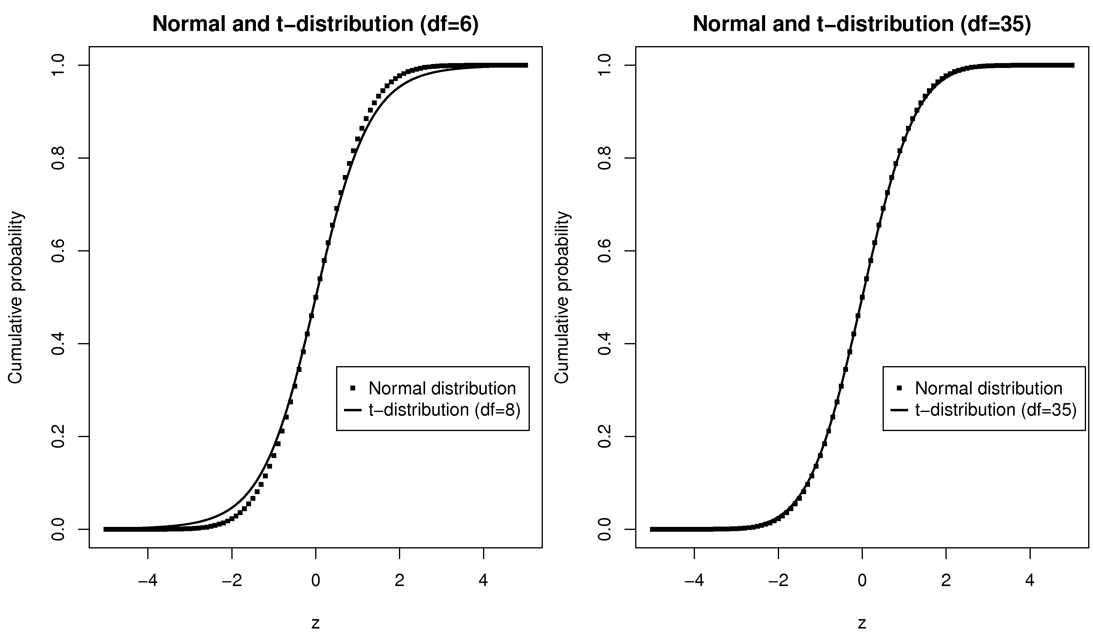
The above source code and figure output shows that the \(t\)-distribution starts being indistinguishable from the normal distribution after about 35 to 40 degrees of freedom. This means that when we deal with large sample sizes (over 40 or 50 samples), then we can use critical values from the normal distribution rather than the \(t\)-distribution. Furthermore, it indicates that our estimate of the variance is a pretty good estimate of the population variance for largish sample sizes.
Question
Explain why tests of differences are insensitive to unit changes. If this were not the case, then one could show a significant difference for a weight-loss supplement when measuring waist size in millimetres, yet show no significant difference when measuring in inches!
Question
A food production facility fills bags with potato chips. The advertised bag weight is 35.0 grams. But, the current bagging system is set to fill bags with a mean weight of 37.4 grams, and this done so that only 1% of bags have a weight of 35.0 grams or less.
Back-calculate the standard deviation of the bag weights, assuming a normal distribution.
Out of 1000 customers, how many are lucky enough to get 40.0 grams or more of potato chips in their bags?
Solution
Calculate the z-value and find which fraction of \(z\) falls at or below 1% of the probability area. From the tables this is -2.326.
Then solve for \(\sigma\):
\[\begin{split}z &= \dfrac{35 - 37.4}{\sigma} = -2.326 \\ \sigma &= \dfrac{35-37.4}{-2.326} = \mathrm{1.03} \text{~grams }\end{split}\]Probability of 40.0 grams of more is the area above the corresponding \(z\)-value:
\[\begin{split}z &> \dfrac{40- 37.4}{1.03} \\ z &> 2.52\end{split}\]The exact answer is
(1 - pnorm(2.52))*1000 = 5.86, though using tables you could use the value corresponding to \(z=2.5\), which is 99.38%, which is the area below that z-value. The area above it is 0.62%, corresponding to 6.2 people. Either 5, 6 or 7 people is an acceptable answer, depending on your rounding error.
Question
A food production facility fills bags with potato chips with an advertised bag weight of 50.0 grams.
The government’s Weights and Measures Act requires that at most 1.5% of customers may receive a bag containing less than the advertised weight. At what setting should you put the target fill weight to meet this requirement exactly? The check-weigher on the bagging system shows the long-term standard deviation for weight is about 2.8 grams.
Out of 100 customers, how many are lucky enough to get 55.0 grams or more of potato chips in their bags?
Solution
Given that it is a long-term standard deviation, we have \(\sigma = 2.8\,\text{grams}\). Calculate the \(z\)-value and find which fraction of \(z\) falls at or below 1.5% of the probability area. From the tables this is \(z = -2.17\) =
qnorm(0.015).Then solve for \(\mu\):
\[\begin{split}z &= \dfrac{50 - \mu}{2.8} = -2.17 \\ \mu &= \mathrm{56.08} \text{~grams}\end{split}\]The check weigher should be set at 56.08 grams.
From the prior answer, we can see many customers will receive a bag with 55.0 grams or more. Probability of 55.0 grams of more is the area area the corresponding \(z\)-value:
\[\begin{split}z &> \dfrac{55 - 56.08}{2.8} \\ z &> -0.385\end{split}\]The exact answer is
(1 - pnorm(-0.385))*100 = 64.98, so around 65 customers out of every 100 (you might have a slightly different number if you used tables to answer your question - make sure you can use the statistical tables to answer this problem too.)
Question
The following confidence interval is reported by our company for the amount of sulphur dioxide measured in parts per billion (ppb) that we send into the atmosphere.
\[123.6\, \text{ppb} \leq \mu \leq 240.2\, \text{ppb}\]
Only \(n=21\) raw data points (one data point measured per day) were used to calculate that 90% confidence interval. A \(z\)-value would have been calculated as an intermediate step to get the final confidence interval, where \(z = \displaystyle \frac{\overline{x} - \mu}{s / \sqrt{n}}\).
What assumptions were made about those 21 raw data points to compute the above confidence interval?
Which lower and upper critical values would have been used for \(z\)? That is, which critical values are used before unpacking the final confidence interval as shown above.
What is the standard deviation, \(s\), of the raw data?
Today’s sulphur dioxide reading is 460 ppb and your manager wants to know what’s going on; you can quickly calculate the probability of seeing a value of 460 ppb, or greater, to help judge the severity of the pollution. How many days in a 365 calendar-day year are expected to show a sulphur dioxide value of 460 ppb or higher?
Explain clearly why a wide confidence interval is not desirable, from an environmental perspective.
Solution
The 21 data points are independent and come from any distribution of finite variance.
From the \(t\)-distribution at 20 degrees of freedom, with 5% in each tail: \(c_t = 1.72\) =
qt(0.95, df=20). The \(t\)-distribution is used because the standard deviation is estimated, rather than being a population deviation.The standard deviation may be calculated from:
\[\begin{split}UB - LB = 240.2 - 123.6 = 2 \times c_t \frac{s}{\sqrt{n}} &= (2)(1.72)\frac{s}{\sqrt{n}} \\ s &= \frac{(116)(\sqrt{n})}{(2)(1.72)} \\ s &= 154.5\, \text{ppb}\end{split}\]Note the very large standard deviation relative to the confidence interval range. This is the reason why so many data points were taken (21), to calculate the average, because the raw data comes from a distribution with such a large variation.
An important note here is the large estimated value for the standard deviation and realized it was so wide, that it would imply the distribution produced values with negative sulphur dioxide concentration (which is physically impossible). However, note that when dealing with large samples (21 in this case), the distinction between the normal and the \(t\)-distribution is minimal. Further, the raw data are not necessarily assumed to be from the normal distribution, they could be from any distribution, including one that is heavy-tailed, such as the F-distribution (see the yellow and green lines in particular).
The probability calculation requires a mean value. Our best guess for the mean is the midpoint of the confidence interval, which is always symmetric about the estimated process mean, \(\overline{x} = \displaystyle \frac{240.2-123.6}{2} + 123.6 = 181.9\). Note that this is not the value for \(\mu\), since \(\mu\) is unknown.
\[z = \frac{460 - 181.9}{154.5} = 1.80\]Probability is
1 - pt(1.8, df=20)= \(1 - 0.9565176 = 0.0434824\), or about \(0.0434824 \times 365 = 15.9\), or about 16 days in the year (some variation is expected, if you have used a statistical table)A wide confidence interval implies that our sulphur dioxide emissions are extremely variable (the confidence interval bounds are a strong function of the process standard deviation). Some days we are putting more pollution up into the air and balancing it out with lower pollution on other days. Those days with high pollution are more environmentally detrimental.

Question
A common unit operation in the pharmaceutical area is to uniformly blend powders for tablets. One such unit is illustrated below (figure taken from Wikipedia). In this question we consider blending an excipient (an inactive magnesium stearate base), a binder, and the active ingredient. The mixing process is tracked using a wireless near infrared (NIR) probe embedded in a V-blender. The mixer is stopped when the NIR spectra become stable. A new supplier of magnesium stearate is being considered that will save $ 294,000 per year.

The 15 most recent runs with the current magnesium stearate supplier had an average mixing time of 2715 seconds, and a standard deviation of 390 seconds. So far you have run 6 batches from the new supplier, and the average mixing time of these runs is 3115 seconds with a standard deviation of 452 seconds. Your manager is not happy with these results so far - this extra mixing time will actually cost you more money via lost production.
The manager wants to revert back to the original supplier, but is leaving the decision up to you; what would be your advice? Show all calculations and describe any additional assumptions, if required.
Solution
This question, similar to most real statistical problems, is open-ended. This problem considers whether a significant difference has occurred. And in many cases, even though there is significant difference, it has to be weighed up whether there is a practical difference as well, together with the potential of saving money (increased profit).
You should always state any assumptions you make, compute a confidence interval for the difference and interpret it.
The decision is one of whether the new material leads to a significant difference in the mixing time. It is desirable, from a production point of view, that the new mixing time is shorter, or at least the same. Some notation:
Assumptions required to compare the two groups:
The individual samples within each group were taken independently, so that we can invoke the central limit theorem and assume these means and standard deviation are normally distributed.
Assume the individual samples within each group are from a normal distribution as well.
Assume that we can pool the variances, i.e. \(\sigma_\text{Before}\) and \(\sigma_\text{After}\) are from comparable distributions.
Using the pooled variance implies that the \(z\)-value follows the \(t\)-distribution.
The mean of each group (before and after) is independent of the other (very likely true).
No other factors were changed, other than the raw material (we can only hope, though in practice this is often not true, and a paired test would eliminate any differences like this).
Calculating the pooled variance:
Computing the z-value for this difference:
The probability of obtaining this value of \(z\) can be found using the \(t\)-distribution at 6 + 15 - 2 = 19 degrees of freedom (because the standard deviation is an estimate, not a population value). Using tables, a value of 0.025, or 2.5% is found (in R, it would be pt(-2.03, df=19) = 0.0283, or 2.83%). At this point one can argue either way that the new excipient leads to longer times, though I would be inclined to say that this probability is too small to be due to chance alone. Therefore there is a significant difference, and we should revert back to the previous excipient. Factors such as operators, and other process conditions could have affected the 6 new runs.
Alternatively, and this is the way I prefer to look at these sort of questions, is to create a confidence interval. At the 95% level, the value of \(c_t\) in the equation below, using 19 degrees of freedom is qt(0.975, df=19) = 2.09 (any value close to this from the tables is acceptable):
\[\begin{split}\begin{array}{rcccl} -c_t &\leq& z &\leq & +c_t \\ (\overline{x}_B - \overline{x}_A) - c_t \sqrt{s_P^2 \left(\frac{1}{n_A} + \frac{1}{n_B}\right)} &\leq& \mu_B - \mu_A &\leq & (\overline{x}_B - \overline{x}_A) + c_t \sqrt{s_P^2 \left(\frac{1}{n_A} + \frac{1}{n_B}\right)}\\ -400 - 2.09 \sqrt{165837 \left(\frac{1}{6} + \frac{1}{15}\right)} &\leq& \mu_B - \mu_A &\leq& -400 + 2.09 \sqrt{165837 \left(\frac{1}{6} + \frac{1}{15}\right)} \\ -400 - 412 &\leq& \mu_B - \mu_A &\leq& -400 + 412 \\ -812 &\leq& \mu_B - \mu_A &\leq& 12 \end{array}\end{split}\]
The interpretation of this confidence interval is that there is no difference between the current and new magnesium stearate excipient. The immediate response to your manager could be “keep using the new excipient”.
However, the confidence interval’s asymmetry should give you pause, certainly from a practical point of view (this is why I prefer the confidence interval - you get a better interpretation of the result). The 12 seconds by which it overlaps zero is so short when compared to average mixing times of around 3000 seconds, with standard deviations of 400 seconds. The practical recommendation is that the new excipient has longer mixing times, so “revert to using the previous excipient”.
One other aspect of this problem that might bother you is the low number of runs (batches) used. Let’s take a look at how sensitive the confidence interval is to that. Assume that we perform one extra run with the new excipient (\(n_A = 7\) now), and assume the pooled variance, \(s_p^2 = 165837\) remains the same with this new run. The new confidence interval is:
So comparing this \(\pm 390\) with 7 runs, to the \(\pm 412\) with 6 runs, shows that the confidence interval shrinks in quite a bit, much more than the 12 second overlap of zero. Of course we don’t know what the new \(\overline{x}_B - \overline{x}_A\) will be with 7 runs, so my recommendation would be to perform at least one more run with the new excipient, but I suspect that the new run would show there to be a significant difference, and statistically confirm that we should “revert to using the previous excipient”.
Question
List an advantage of using a paired test over an unpaired test. Give an example, not from the notes, that illustrates your answer.
Solution
One primary advantage of pairing is that any systematic difference between the two groups (A and B) is eliminated. For example, a bias in the measurement will cancel out when calculating the pairs of differences. Any example is suitable as an answer: e.g. laboratory miscalibration; an offset in an on-line sensor, etc.
Other advantages are that the raw data do not need to be normally distributed, only the paired differences.
Another advantage is that randomization of the trials is required in the unpaired case (often a costly extra expense), whereas in the paired case, we only need to be sure the pairs are independent of each other (that’s much easier to assume, and often true). For example testing drug A and B on a person, some time apart. The pairs are run on the same person, but each person in the drug trial is independent of the other.
Question
An unpaired test to distinguish between group A and group B was performed with 18 runs: 9 samples for group A and 9 samples for group B. The pooled variance was 86 units.
Also, a paired test on group A and group B was performed with 9 runs. After calculating the paired differences, the variance of these differences was found to be 79 units.
Discuss, in the context of this example, an advantage of paired tests over unpaired tests. Assume 95% confidence intervals, and that the true result was one of “no significant difference between method A and method B”. Give numeric values from this example to substantiate your answer.
Solution
One advantage of the paired test is that often a fewer number of samples are required to obtain a more sensitive result than when analyzing the data as from two distinct, unpaired groups.
Construct the confidence interval for both cases, substitute in these values and then compare the confidence intervals. The equations for both confidence intervals are derived directly from the \(z\)-value.
Unpaired case:
The \(c_t\) value for the unpaired case is from the \(t\)-distribution with 16 degrees of freedom, a value of around 2.12.
Paired case:
In this case the vector of differences is \(w\), and by the central limit theorem it is distributed as \(w \sim \mathcal{N}\left( \mu_{B-A} , \sigma_w^2/n \right)\), but we use the estimated variance, \(s_w^2\) instead.
\[\begin{split}\begin{array}{rcccl} - c_t &\leq& \dfrac{\overline{w} - \mu_{B-A}}{s_w / \sqrt{n}} &\leq & +c_t\\ \\ \overline{w} - c_t \dfrac{s_w}{\sqrt{n}} &\leq& \mu_w &\leq & \overline{w} + c_t \dfrac{s_w}{\sqrt{n}} \\ \overline{w} - 2.3 \dfrac{\sqrt{79}}{\sqrt{9}} &\leq& \mu_w &\leq & \overline{w} + 2.3 \dfrac{\sqrt{79}}{\sqrt{9}} \\ \overline{w} - 6.81 &\leq& \mu_w &\leq& \overline{w} + 6.81 \end{array}\end{split}\]
The \(c_t\) value for the paired case is from the \(t\)-distribution with 8 degrees of freedom, a value of around 2.3.
The key result of this question is that the confidence interval for the paired case is tighter (narrower) than the confidence interval from the unpaired case. Given that the true result was one of no significant difference, it implies that \(\mu_A = \mu_B\) and that \(\mu_w = 0\). The tighter confidence interval comes purely from the fact that the standard deviation used for the paired case is smaller, \(\sqrt{\dfrac{79}{9}}\) vs the \(\sqrt{86 \left(\dfrac{1}{9} + \dfrac{1}{9}\right)}\) from the unpaired case. This is not due to the variances, since \(\sqrt{86} \approx \sqrt{79}\), i.e. (9.27 vs 8.88), but rather due to the fact that that unpaired standard deviation is multiplied by \(\sqrt{2/9}\), while the paired standard deviation is multiplied by \(\sqrt{1/9}\).
So while the \(c_t\) value for the paired case is actually larger (widening the confidence interval due to the fewer degrees of freedom), the overall effect is that the paired confidence interval is narrower than the unpaired confidence interval. This result holds for most cases of paired and unpaired studies, though not always.
Question
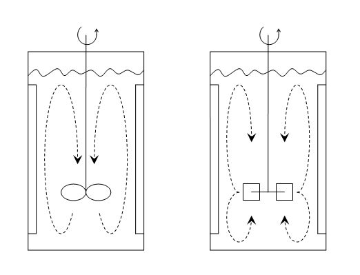
You are convinced that a different impeller (mixing blade) shape for your tank will lead to faster, i.e. shorter, mixing times. The choices are either an axial blade or a radial blade, as shown in this figure from Wikipedia.
Before obtaining approval to run some experiments, your team wants you to explain how you will interpret the experimental data. Your reply is that you will calculate the average mixing time from each blade type and then calculate a confidence interval for the difference. A team member asks you what the following 95% confidence intervals would mean:
\(-453 \text{~seconds} \leq \mu_{\text{Axial}} - \mu_{\text{Radial}} \leq 390 \text{~seconds}\)
\(-21 \text{~seconds} \leq \mu_{\text{Axial}} - \mu_{\text{Radial}} \leq 187 \text{~seconds}\)
For both cases (a) explain what the confidence interval means in the context of this experiment, and (b) whether the recommendation would be to use radial or axial impellers to get the shortest mixing time.
3. Now assume the result from your experimental test was \(-21 \text{~seconds} \leq \mu_{\text{Axial}} - \mu_{\text{Radial}} \leq 187 \text{~seconds}\); how can you make the confidence interval narrower?
Solution
This confidence interval spans zero, and nearly symmetrically. This implies the population difference is likely zero, while the symmetry implies their is no preference either way: the difference in mixing times is as low as -453 seconds or as high as 390 seconds. The recommendation is that either the axial or radial impeller could be used, with no expected long-term difference. Use the cheaper impeller; or use the axial impeller if the costs are the same (only because of the very slight imbalance in the CI). Note that there is a 5% chance that the confidence interval does not contain the true difference.
This confidence interval also spans zero, so there is no statistical difference between the two impellers. However the CI does not span zero symmetrically. The asymmetry of the interval makes me much less comfortable recommending that there is no practical difference between the impellers. It often happens in these cases that by removing a single data point that the confidence interval does not span zero anymore. In this case I would recommend either impeller, but if there is no cost difference, I would prefer the radial impeller, as it might have shorter mixing times, especially if the confidence interval quoted here is only due to one observation. A careful review of the raw data would be useful in this case.
The confidence interval can be made narrower in 2 ways (as long as the sample mean and sample standard deviation remain stable):
Use more data points, \(n\) in both groups.
Choose a lower degree of confidence, e.g. 90% instead of 95%, which is really just an artificial reduction of the interval.
One can also reduce the interval by shrinking the standard deviation, but that’s usually not a practical possibility. You cannot perform a paired test, as you only have one mixing tank.
Interpreting confidence intervals
Recall the definition of the confidence interval is subtle: it says 95% of the time, the upper and lower bounds of the confidence interval contain the true value of the parameter; it does not say there is a 95% probability the true value of the parameter lies inside the bounds. That last part is incorrect because it implies the true value of the parameter can vary, which it can’t: the true parameter value is fixed, only the bounds change.
Question
The paper by PJ Rousseeuw, “Tutorial to Robust Statistics”, Journal of Chemometrics, 5, 1-20, 1991 discusses the breakdown point of a statistic.
Describe what the breakdown point is, and give two examples: one with a low breakdown point, and one with a high breakdown point. Use a vector of numbers to help illustrate your answer.
What is an advantage of using robust methods over their “classical” counterparts?
Solution
PJ Rousseeuw defines the breakdown point on page 3 of his paper as “… the smallest fraction of the observations that have to be replaced to make the estimator unbounded. In this definition one can choose which observations are replaced, as well as the magnitude of the outliers, in the least favourable way”.
A statistic with a low breakdown point is the mean, of the \(n\) values used to calculate the mean, only 1 needs to be replaced to make the estimator unbounded; i.e. its breakdown point is \(1/n\). The median though has a breakdown point of 50%, as one would have to replace 50% of the \(n\) data points in the vector before the estimator becomes unbounded.
Use this vector of data as an example: \([2, 6, 1, 9151616, -4, 2]\). The mean is 1525270, while the median is 2.
Robust methods are insensitive to outliers, which is useful when we need a measure of location or spread that is calculated in an automated way. It is increasingly prevalent to skip out the “human” step that might have detected the outlier, but our data sets are getting so large that we can’t possibly visualize or look for outliers manually anymore.
As described in the above paper by Rousseeuw, robust methods also emphasize outliers. Their “lack of sensitivity to outliers” can also be considered an advantage.
Question
Why are robust statistics, such as the median or MAD, important in the analysis of modern data sets? Explain, using an example, if necessary.
What is meant by the break-down point of a robust statistic? Give an example to explain your answer.
Solution
Data sets you will have to deal with in the workplace are getting larger and larger (lengthwise), and processing them by trimming outliers (see Question 5 later) manually is almost impossible. Robust statistics are a way to summarize such data sets without point-by-point investigation.
This is especially true for automatic systems that you will build that need to (a) acquire and (b) process the data to then (c) produce meaningful output. These systems have to be capable of dealing with outliers and missing values.
The breakdown point is the number of contaminating data points required before a statistic (estimator) becomes unbounded, i.e. useless. For example, the mean requires only 1 contaminating value, while the median requires 50% + 1 data points before it becomes useless.
Consider the sequence \([2, 6, 1, 91511, -4, 2]\). The mean is 15253, while the median is 2, which is a far more useful estimate of the central tendency in the data.
Question
Recall that \(\mu = \mathcal{E}(x) = \frac{1}{N}\sum{x}\) and \(\mathcal{V}\left\{x\right\} = \mathcal{E}\left\{ (x - \mu )^2\right\} = \sigma^2 = \frac{1}{N}\sum{(x-\mu)^2}\).
What is the expected value thrown of a fair, 12-sided dice?
What is the expected variance of a fair, 12-sided dice?
Simulate 10,000 throws in a software package (R, MATLAB, or Python) from this dice and see if your answers match those above. Record the average value from the 10,000 throws, call that average \(\overline{x}\).
Repeat the simulation 10 times, calculating the average value of all the dice throws. Calculate the mean and standard deviation of the 10 \(\overline{x}\) values and comment whether the results match the theoretically expected values.
Solution
The objective of this question is to recall basic probability rules.
Each value on the dice is equally probable, so the expected value thrown will be:
\[\mathcal{E}(X) = \sum_{i=1}^{12}x_{i}P(x_{i}) = P(x) \sum_{i=1}^{12} x_{i} = \frac{1}{12} \left( 1 + 2 + \cdots + 12 \right) = \bf{6.5}\]This value is the population mean, \(\mu\).
Continuing the notation from the above question we can derive the expected variance as,
\[\mathcal{V}(X) = \frac{1}{N}\sum_i^{12}{(x_i - \mu)^2} = \frac{1}{12} \cdot \left[ (1 - 6.5)^2 + (2 - 6.5)^2 + \ldots + (12 - 6.5)^2 \right] \approx \bf{11.9167}\]Simulating 10,000 throws corresponds to 10,000 independent and mutually exclusive random events, each with an outcome between 1 and 12. The sample mean and variance from my sample was calculated using this code in R:
\[\begin{split}\overline{x} &= 6.5219\\ s^2 &= 12.03732\end{split}\]S, 13 lines
# Set the random seed to a known point, to allow
# us to duplicate pseudorandom results
set.seed(13)

x.data <- as.integer(runif(10000, 1, 13))

# Verify that it is roughly uniformly distributed
# across 12 bins
hist(x.data, breaks=seq(0,12))

x.mean <- mean(x.data)
x.var <- var(x.data)
c(x.mean, x.var)
Repeating the above simulation 10 times (i.e. 10 independent experiments) produces 10 different estimates of \(\mu\) and \(\sigma^2\). Note, your answer should be slightly different, and different each time you run the simulation.
S, 32 lines
N <- 10
n <- 10000
x.mean <- numeric(N)
x.var <- numeric(N)
for (i in 1:N) {
  x.data <- as.integer(runif(n, 1, 13))
  x.mean[i] <- mean(x.data)
  x.var[i] <- var(x.data)
}

x.mean
# [1] 6.5527 6.4148 6.4759 6.4967 6.4465
# [6] 6.5062 6.5171 6.4671 6.5715 6.5485

x.var
# [1] 11.86561 11.84353 12.00102 11.89658 11.82552
# [6] 11.83147 11.95224 11.88555 11.81589 11.73869

# You should run the code several times and verify whether
# the following values are around their expected, theoretical
# levels.  Some runs should be above, and other runs below
# the theoretical values.
# This is the same as increasing "N" in the first line.

# Is it around 6.5?
mean(x.mean)

# Is it around 11.9167?
mean(x.var)

# Is it around \sigma^2 / n = 11.9167/10000 = 0.00119167 ?
var(x.mean)
Note that each \(\overline{x} \sim \mathcal{N}\left(\mu, \sigma^2/n \right)\), where \(n = 10000\). We know what \(\sigma^2\) is in this case: it is our theoretical value of 11.92, calculated earlier, and for \(n=10000\) samples, our theoretical expectation is that \(\overline{x} \sim \mathcal{N}\left(6.5, 0.00119167\right)\).
Calculating the average of those 10 means, let’s call that \(\overline{\overline{x}}\), shows a value close to 6.5, the theoretical mean.
Calculating the variance of those 10 means shows a number around 0.00119167, as expected.
Question
Removed. Was a duplicate of a prior question (number 13).
Question
At the 95% confidence level, for a sample size of 7, compare and comment on the upper and lower bounds of the confidence interval that you would calculate if:
you know the population standard deviation
you have to estimate it for the sample.
Assume that the calculated standard deviation from the sample, \(s\) matches the population \(\sigma = 4.19\).
As a follow up, overlay the probability distribution curves for the normal and \(t\)-distribution that you would use for a sample of data of size \(n=7\).
Repeat part of this question, using larger sample sizes. At which point does the difference between the \(t\)- and normal distributions become practically indistinguishable?
What is the implication of this?
Solution
This question aims for you to prove to yourself that the \(t\)-distribution is wider (more broad) than the normal distribution, and as a result, the confidence interval is wider as well. This is because we are less certain of the data’s spread when using the estimated variance.
The confidence intervals are:
\[\begin{split}\begin{array}{rcccl} - c_n &\leq& \displaystyle \frac{\overline{x} - \mu}{\sigma/\sqrt{n}} &\leq & c_n\\ \\ - c_t &\leq& \displaystyle \frac{\overline{x} - \mu}{s/\sqrt{n}} &\leq & c_t \end{array}\end{split}\]The 95% region spanned by the \(t\)-distribution with 6 degrees of freedom has upper and lower limits at \(c_t = \pm\)
qt((1-0.95)/2, df=6), i.e. from -2.45 to 2.45. The equivalent 95% region spanned by the normal distribution is \(c_n = \pm\)qnorm((1-0.95)/2), spanning from z=-1.96 to z=1.96. Everything else in the center of the 2 inequalities is the same, so we only need to compare \(c_t\) and \(c_n\).The question asked to overlay the probability distributions (not cumulative probability distributions):

where the above figure was generated with the R-code:
Python, 16 lines
# The normal and t densities for a sample of 7, so 6 degrees of freedom.
import numpy as np
import plotly.graph_objects as go
from scipy import stats

n = 7
z = np.arange(-5, 5.001, 0.01)

fig = go.Figure()
fig.add_scatter(x=z, y=stats.norm.pdf(z), mode="lines",
                name="Normal distribution")
fig.add_scatter(x=z, y=stats.t.pdf(z, df=n - 1), mode="lines",
                line_dash="dash", name=f"t-distribution (df={n - 1})")
fig.update_layout(xaxis_title_text="z",
                  yaxis_title_text="Normal and t-distributions")
fig.show()
or the equivalent in R:
S, 9 lines
n <- 7
z <- seq(-5, 5, 0.01)
prob.norm <- dnorm(z)
prob.t <- dt(z, df=n-1)

plot(z, prob.norm, type="l", ylab="Normal and t-distributions", lwd=2)
lines(z, prob.t, lty=8, lwd=2)  # dashed line
legend(x=1.35, y=0.25, legend=c("Normal distribution", "t-distribution"),
       lty=c(1,8), lwd=c(2,2))
Repeated use of the above code, but changing \(n\), shows that little practical difference between the distributions with as few as \(n=20\) samples. After \(n=40\) and especially \(n=60\), there is almost no theoretical difference between them.
This implies that when we do any analysis of large samples of data, say \(n>50\), and if those data are independently sampled, then we can just use the normal distribution’s critical value (e.g. the \(\pm 1.96\) value for 95% confidence, which you now know from memory), instead of looking up the \(t\)-distribution’s values.
Since the wider values from the \(t\)-distribution reflect our uncertainty in using an estimate of the variance, rather than the population variance, this result indicates that our estimated variances are a good estimate of the population variance for largish sample sizes.
Question
Engineering data often violate the assumption of independence. In this question you will create (simulate) sequences of autocorrelated data, i.e. data that lack independence, and investigate how lack of independence affects our results.
The simplest form of autocorrelation is what is called lag-1 autocorrelation, when the series of values, \(x_k\) is correlated with itself only 1 step back in time, \(x_{k-1}\):
The \(a_k\) value is a random error and for this question let \(a_k \sim \mathcal{N}\left(\mu=0, \sigma^2 = 25.0 \right)\).
Create 3 sequences of autocorrelated data with:
A: \(\qquad \phi = +0.7\) (positively correlated)
B: \(\qquad \phi = 0.0\) (uncorrelated data)
C: \(\qquad \phi = -0.6\) (negatively correlated)
For case A, B and C perform the following analysis. Repeat the following 1000 times (let \(i = 1, 2, \ldots, 1000\)):
Create a vector of 100 autocorrelated \(x\) values using the above formula, using the current level of \(\phi\)
Calculate the mean of these 100 values, call it \(\overline{x}_i\) and store the result
At this point you have 1000 \(\overline{x}_i\) values for case A, another 1000 \(\overline{x}_i\) values for case B, and similarly for case C. Now answer these questions:
Assuming independence, which is obviously not correct for 2 of the 3 cases, nevertheless, from which population should \(\overline{x}\) be from, and what are the 2 parameters of that population?
Now, using your 1000 simulated means, estimate those two population parameters.
Compare your estimates to the theoretical values.
Comment on the results, and the implication of this regarding tests of significance (i.e. statistical tests to see if a significant change occurred or not).
Solution
We expect that case B should match the theoretical case the closest, since data from case B are truly independent, since the autocorrelation parameter is zero. We expect case A and C datasets, which violate that assumption of independence, to be biased one way or another. This question aims to see how they are biased.
S, 21 lines
nsim <- 1000            # Number of simulations
x.mean <- numeric(nsim) # An empty vector to store the results

set.seed(37)            # so that you can reproduce these results
for (i in 1:nsim)
{
    N <- 100            # number of points in autocorrelated sequence
    phi <- +0.7         # ** change this line for case A, B and C **
    spread <- 5.0       # standard deviation of random variables
    x <- numeric(N)
    x[1] = rnorm(1, mean=0, sd=spread)
    for (k in 2:N){
       x[k] <- phi*x[k-1] + rnorm(1, mean=0, sd=spread)
    }
    x.mean[i] <- mean(x)
}
theoretical <- sqrt(spread^2/N)

# Show some output to the user
c(theoretical, mean(x.mean), sd(x.mean))
You should be able to reproduce the results I have below, because the above code uses the set.seed(...) function, which forces R to generate random numbers in the same order on my computer as yours (as long as we all use the same version of R).
Case A:
0.50000000, 0.00428291, 1.65963302Case B:
0.50000000, 0.001565456, 0.509676562Case C:
0.50000000, 0.0004381761, 0.3217627596
The first output is the same for all 3 cases: this is the theoretical standard deviation of the distribution from which the \(\overline{x}_i\) values come: \(\overline{x}_i \sim \mathcal{N}\left(\mu, \sigma^2/N \right)\), where \(N=100\), the number of points in the autocorrelated sequence. This result comes from the central limit theorem, which tells us that \(\overline{x}_i\) should be normally distributed, with the same mean as our individual \(x\)-values, but have smaller variance. That variance is \(\sigma^2/N\), where \(\sigma\) is the variance of the distribution from which we took the raw \(x\) values. That theoretical variance value is \(25/100\), or theoretical standard deviation of \(\sqrt{25/100} = \bf{0.5}\).
But, the central limit theorem only has one crucial assumption: that those raw \(x\) values are independent. We intentionally violated this assumption for case A and C.
We use the 1000 simulated values of \(\overline{x}_i\) and calculate the average of the 1000 \(\overline{x}_i\) values and the standard deviation of the 1000 \(\overline{x}_i\) values. Those are the second and third values reported above.
We see in all cases that the mean of the 1000 values nearly matches 0.0. If you run the simulations again, with a different seed, you will see it above zero, and sometimes below zero for all 3 cases. So we can conclude that lack of independence does not affect the estimated mean.
The major disagreement is in the variance though. Case B matches the theoretical variance; data that are positively correlated have an inflated standard deviation, 1.66; data that are negatively correlated have a deflated standard deviation, 0.32 when \(\phi=-0.6\).
This is problematic for the following reason. When doing a test of significance, we construct a confidence interval:
We use an estimated standard deviation, \(s\), whether that is found from pooling the variances or found separately (it doesn’t really matter), but the main problem is that \(s\) is not accurate when the data are not independent:
For positive correlations (quite common in industrial data): our confidence interval will be too wide, likely spanning zero, indicating no statistical difference, when in fact there might be one.
For negative correlations (less common, but still seen in practice): our confidence interval will be too narrow, more likely to indicate there is a difference.
The main purpose of this question is for you to see how use to understand what happens when a key assumption is violated. There are cases when an assumption is violated, but it doesn’t affect the result too much.
In this particular example there is a known theoretical relationship between \(\phi\) and the inflated/deflated variance that can be derived (with some difficulty). But in most situations the affect of violating assumptions is too difficult to derive mathematically, so we use computer power to do the work for us: but then we still have to spend time thinking and interpreting the results.
Question
Sulphur dioxide is a byproduct from ore smelting, coal-fired power stations, and other sources.
These 11 samples of sulphur dioxide, SO2, measured in parts per billion [ppb], were taken from our plant. Environmental regulations require us to report the 90% confidence interval for the mean SO2 value.
\[180, \,\, 340, \,\,220, \,\,410, \,\,101, \,\,89, \,\,210, \,\,99, \,\,128, \,\,113, \,\,111\]
What is the confidence interval that must be reported, given that the sample average of these 11 points is 181.9 ppb and the sample standard deviation is 106.8 ppb?
Why might Environment Canada require you to report the confidence interval instead of the mean?
Solution
From the central limit theorem, assuming the 11 values are independent, the mean SO2 value, \(\overline{x} \sim \mathcal{N}\left\{\mu, \sigma^2/n \right\}\), where \(\mu\) and \(\sigma\) are the distribution from which the raw values come.
Using an estimate for \(\sigma = \hat{s} = 106.8\) we can construct the \(z\)-value and confidence interval. \(z\) will be \(t\)-distributed with \(n-1 = 10\) degrees of freedom, so \(c_t = 1.81\) At the 90% confidence level we can then write:
\[\begin{split}\begin{array}{rcccl} - c_t &\leq& \displaystyle \frac{\overline{x} - \mu}{s/\sqrt{n}} &\leq & +c_t\\ \overline{x} - c_t \dfrac{s}{\sqrt{n}} &\leq& \mu &\leq& \overline{x} + c_t\dfrac{s}{\sqrt{n}} \\ 181.9 - 1.81 \times \frac{106.8}{\sqrt{11}} &\leq& \mu &\leq& 181.9 + 1.81 \times \frac{106.8}{\sqrt{11}} \\ 123.6 \,\,\text{ppb} &\leq& \mu &\leq& 240.2 \,\,\text{ppb} \end{array}\end{split}\]Environment Canada may require the confidence interval since in addition to providing an estimate of the mean (just the midpoint of the CI), it also provides an estimate of the spread – variability in your process – if \(n\) is known, without requiring access to the raw data.
A wide CI gives an indication that you might in fact be polluting too much on some days, and compensating on others, which is not desirable. The confidence interval’s width can also be compared between plants to find the most variable polluters.
Question
A concrete slump test is used to test for the fluidity, or workability, of concrete. It’s a crude, but quick test often used to measure the effect of polymer additives that are mixed with the concrete to improve workability.
The concrete mixture is prepared with a polymer additive. The mixture is placed in a mold and filled to the top. The mold is inverted and removed. The height of the mold minus the height of the remaining concrete pile is called the “slump”, as shown in this figure from Wikipedia.

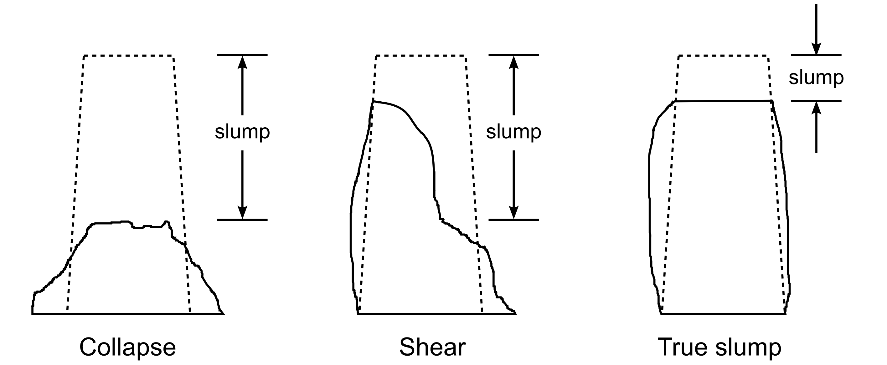
Your company provides the polymer additive, and you are developing an improved polymer formulation, call it B, that hopefully provides the same slump values as your existing polymer, call it A. Formulation B costs less money than A, but you don’t want to upset, or lose, customers by varying the slump value too much.
You have a single day to run your tests (experiments). Preparation, mixing times, measurement and clean up take 1 hour, only allowing you to run 10 experiments. Describe all precautions, and why you take these precautions, when planning and executing your experiment. Be very specific in your answer (use bullet points).
The following slump values were recorded over the course of the day:
Additive
Slump value [cm]
A
5.2
A
3.3
B
5.8
A
4.6
B
6.3
A
5.8
A
4.1
B
6.0
B
5.5
B
4.5
What is your conclusion on the performance of the new polymer formulation (system B)? Your conclusion must either be “send the polymer engineers back to the lab” or “let’s start making formulation B for our customers”. Explain your choice clearly.
To help you, \(\overline{x}_A = 4.6\) and \(s_A = 0.97\). For system B: \(\overline{x}_B = 5.62\) and \(s_B = 0.69\).
Note: In your answer you must be clear on which assumptions you are using and, where necessary, why you need to make those assumptions.
Describe the circumstances under which you would rather use a paired test for differences between polymer A and B.
What are the advantage(s) of the paired test over the unpaired test?
Clearly explain which assumptions are used for paired tests, and why they are likely to be true in this case?
The slump tests were actually performed in a paired manner, where pairing was performed based on the cement supplier. Five different cement suppliers were used:
Supplier
Slump value [cm] from A
Slump value [cm] from B
1
5.2
5.8
2
3.3
4.5
3
4.6
6.0
4
5.8
5.5
5
4.1
6.2
Use these data, and provide, if necessary, an updated recommendation to your manager.
Solution
The basic rule is to control what you can and randomize against what you cannot. You should have mentioned some of these items:
Control: clean equipment thoroughly between runs.
Control: other factors that might affect the slump: temperature, humidity.
Control: ensure the same person prepares all mixtures, or randomize the allocation of people if you have to use more than 1 person. Don’t let person 1 prepare all the A mixtures and person 2 the B mixtures.
Control: mixing times and how the mixture is created could have an effect. This should ideally be done by the same person.
Randomize the order of all the A and B experiments: don’t run all the A’s, then all the B’s, as that will confound with other factors. For example, even though temperature might vary during the day, if we randomize the run order, then we prevent temperature from affecting the results.
Use raw materials (cement, binder, other ingredients) from all possible suppliers. And the supplier raw materials should be representative.
We will initially assume that \(\mu_A = \mu_B\), in other words, the outcome is “let’s start making formulation B for our customers”. We will construct a confidence interval for the difference, \(\mu_B - \mu_A\) and interpret that CI.
Assume the slump values within each group are independent, which will be true if we take the precautions above. We do this because then we can use the central limit theorem (CLT) to state \(\overline{x}_A \sim \mathcal{N}\left(\mu_A, \sigma_A^2/n_A \right)\) and that \(\overline{x}_B \sim \mathcal{N}\left(\mu_B, \sigma_B^2/n_B \right)\).
Note: we don’t require the samples within each group to be normally distributed.
Assume the variances are the same: \(\sigma_A^2 = \sigma_B^2 = \sigma^2\): this is required to simplify the next step.
Assume the \(\overline{x}_A\) and \(\overline{x}_B\) means are independent. This allows us to calculate a variance value, \(\mathcal{V} \left\{\overline{x}_B - \overline{x}_A \right\}\) from which we can create a \(z\)-value for \(\mu_B - \mu_A\):
\[z = \frac{\left(\overline{x}_B - \overline{x}_A \right) - \left(\mu_B - \mu_A\right)}{\sqrt{\mathcal{V} \left\{\overline{x}_B - \overline{x}_A \right\}}}\]That denominator variance can be written as:
\[\begin{split}\mathcal{V} \left\{\overline{x}_B - \overline{x}_A\right\} &= \mathcal{V} \left\{\overline{x}_B \right\} + \mathcal{V} \left\{\overline{x}_A\right\}\\ &= \sigma^2\left(\frac{1}{n_B} + \frac{1}{n_A} \right)\end{split}\]using our previous assumption that the variances are equal. We can verify this with an \(F\)-test, but won’t do it here.
Because we do not have an external estimate of the variance, \(\sigma^2\), available, we must assume a good estimate for it can be found by pooling the estimated variances of the group A and B samples (which requires our equal variance assumption from earlier).
\[\begin{split}s_P^2 &= \frac{4s_A^2 + 4s_B^2}{4 + 4} \\ s_P^2 &= \frac{4(0.97)^2 + 4(0.69)^2}{4 + 4} = 0.709\\\end{split}\]This pooling also gives us 8 degrees of freedom for the \(t\)-distribution, which is how the \(z\)-value is distributed.
Using that \(z\)-value and filling our assumed difference of zero for the true means, we can construct a 95% confidence interval:
\[\begin{split}\begin{array}{rcccl} -c_t &\leq& z &\leq & +c_t \\ (\overline{x}_B - \overline{x}_A) - c_t \sqrt{s_P^2 \left(\frac{1}{n_B} + \frac{1}{n_A}\right)} &\leq& \mu_B - \mu_A &\leq & (\overline{x}_B - \overline{x}_A) + c_t \sqrt{s_P^2 \left(\frac{1}{n_B} + \frac{1}{n_A}\right)}\\ 1.02 - 2.3 \sqrt{0.709 \left(\frac{1}{5} + \frac{1}{5}\right)} &\leq& \mu_B - \mu_A &\leq& 1.02 + 2.3 \sqrt{0.709 \left(\frac{1}{5} + \frac{1}{5}\right)} \\ -0.21 &\leq& \mu_B - \mu_A &\leq& 2.2 \end{array}\end{split}\]The statistical conclusion is that there is no difference between formulation A and B, since the CI spans zero. However, the practical interpretation is that the CI only just contains zero, and this should cause us to stop, and really consider the risk of the statistical conclusion.
If one of the data points were in error just slightly, or if we ran a single additional experiment, it is quite possible the CI will not span zero anymore. In my mind, this risk is too great, and we risk upsetting the customers.
So my conclusion would be to “send the polymer engineers back to the lab” and have them improve their formulation until that CI spans zero more symmetrically.
A paired test should be used when there is something is common within pairs of samples in group A and B, but that commonality does not extend between the pairs. Some examples though you could have mentioned:
Pairing is appropriate: person 1 mixes polymer for test A and B; person 2 mixes polymer for test A and B (but with different time and agitation level that person 2); person 3 mixes … etc Pairing not appropriate: person 1 mixes all the polymer A samples; person 2 mixes all the polymer B samples (pairing won’t fix this, and even the unpaired results will be inaccurate - see precautions mentioned above). Pairing appropriate: you only have enough cement and raw materials to create the concrete mixture for 2 samples: one for A and one for B. You repeat this 5 times, each time using a different supplier’s raw materials.
In other words, pairing is appropriate when there is something the prevents the \(\overline{x}_A\) and \(\overline{x}_B\) quantities from being independent.
The one advantage of the paired test is that it will cancel out any effect that is common between the pairs (whether that effect actually affects the slump value or not). Pairing is a way to guard against potential effect.
This makes the test more sensitive to the difference actually being tested for (formulation A vs B) and prevents confounding from the effect we are not testing for (suppliers’ raw material).
Unpaired tests, but with randomization will only prevent us from being misled, however that supplier effect is still present in the 10 experimental values. The 5 difference values used in the paired tests will be free from that effect.
Pairing requires/assumes that the paired objects have something in common (e.g. a common bias due to the cement raw material). This common bias will be cancelled out once we calculate the difference in measurements.
The difference values calculated, \(w_i\), are assumed to be independent. This is likely true in this case because each raw material supplier is different (unrelated) to the other.
If the differences are independent, then the central limit theorem can be safely assumed so that the average of these differences, \(\overline{w} \sim \mathcal{N}\left(\mu_w, \sigma_w^2/n \right)\).
The 5 difference values are \(w_i = \left[ 0.6,\,\, 1.2,\,\, 1.4,\,\, -0.3, \,\, 2.1 \right]\) and the average difference value is \(\overline{w} = 1\) and its estimated variance is \(s_w^2 = 0.815\).
Create the \(z\)-value against the \(t\)-distribution with 4 degrees of freedom (\(c_t = 2.78\)), at the 95% confidence level, and unpack it into a confidence interval.
\[\begin{split}\begin{array}{rcccl} -c_t &\leq& z &\leq & +c_t \\ \overline{w} - c_t \sqrt{\frac{s^2}{n}} &\leq& \mu_w &\leq & \overline{w} + c_t \sqrt{\frac{s^2}{n}}\\ 1 - 2.78 \sqrt{\frac{0.815}{4}} &\leq& \mu_w &\leq & 1 + 2.78 \sqrt{\frac{0.815}{4}}\\ -0.12 &\leq& \mu_w &\leq & 2.12 \end{array}\end{split}\]The interpretation is that the true difference in slump, \(\mu_w\), when accounting for variation from the cement raw material, is again not statistically significant, at the 95% confidence level.
Practically though, there is a bit of a risk, due to the imbalance (asymmetry) in the confidence interval. It would be reluctant to hinge my company’s profitability on this result, especially with the fact that there are only 4 experiments. So my personal conclusion would be to still “send the polymer engineers back to the lab”.
Question
You are planning a series of experiments to test alternative conditions in a store and see which conditions lead to higher sales.
Which practical steps would you take to ensure independence in the experimental data, when investigating:
adjustable halogen lighting: A = soft and dim lighting and B = brighter lighting
alternative shelving: A = solid white metal shelves and B = commercial stainless steel racking
Solution
By Cameron DiPietro and Andrew Haines (2012 class)
Randomization is expensive and inconvenient; however, the high cost is to ensure that the results attained in each study are not affected by unmeasured disturbances. We also have to take care to control measured disturbances as far as possible.
To ensure independence when investigating adjustable halogen lighting: A = soft and dim lighting and B = brighter lighting, the following experiments and conditions may be run:
All light fixtures are changed correctly during the swap from A to B and the same scenario from B to A
Keep prices of all products the same during days with A lighting and days with B lighting
Do not inform customers of A to B swap or B to A swap in lighting
Ensure product quality
Use the same amount of voltage throughout the store for each lighting arrangement
Keep the store stocked the same for everyday during experiment
Use random days for each light fixture
Maintain the same advertisements for the store during the study
Do not inform employees of lighting swaps to ensure identical employee to customer relationships
Compensate for any holiday or unexpected short days of store hours
Have employees work randomized shifts to ensure no patterns in employees moods during light fixture swaps
Employees have the same mindset to customers (if a retail business) during both A and B lighting arrangements
Assume all data from A and B light fixtures have identical population variance
If lighting A and B are installed simultaneously, then it might be possible to even run different tests during the day, randomly allocated.
To ensure independence when investigating alternative shelving: A = solid white metal shelves and B = commercial stainless steel racking, the following experiments and conditions may be run:
Shelving size remains the same and in the same location
Identical product placement on both shelves A and B, if possible
Being able to control everything other than the variable being studied of shelves
Distances between shelves identical
Ensure employees have the same mindset during each customer visit
Identical number of items per shelf
Same shelf distances from checkout
Clean each shelf in the same manner for both A and B
Keep prices and sales the same throughout the study period
Clearly the shelf study cannot be easily implemented, since the logistics of unstocking, removing shelf A, replacing with shelf B and restocking them is extremely costly.
One thing to consider in such cases is to run the experiments in two separate stores that are as similar as possible in all other respects (e.g. built in the area with similar profiles of customers, similar store layout, etc.).
Question
This question gives you exposure to analyzing a larger data set than seen in the preceding questions.
Your manager has asked you to describe the flow rate characteristics of the overhead stream leaving the top of the distillation column at your plant. You are able to download one month of data, available from this website, from 1 March to 31 March, taken at one minute intervals to answer this question.