
 Download PDF of entire book
4.7. Least squares model analysis
Once we have fitted the \(b_0\) and \(b_1\) terms using the data and the equations from the prior section, it is of interest to know how well the model performed. That is what this section is about. In particular:
Analysis of variance: breaking down the data’s variability into components
Confidence intervals for the model coefficients, \(b_0\) and \(b_1\)
Prediction error estimates for the \(y\)-variable
We will also take a look at the interpretation of the software output.
In order to perform the second part we need to make a few assumptions about the data, and if the data follow those assumptions, then we can derive confidence intervals for the model parameters.
4.7.1. The variance breakdown
Recall that variability is what makes our data interesting. Without variance (i.e. just flat lines) we would have nothing to do. The analysis of variance is just a tool to show how much variability in the \(y\)-variable is explained by:
Doing nothing (no model: this implies \(\hat{y} = \overline{y}\))
The model (\(\hat{y}_i = b_0 + b_1 x_i\))
How much variance is left over in the errors, \(e_i\)
These components must add up to the total variance we started with. By definition, the variance is computed about a mean, so the “doing nothing” case explains no variance: its prediction is the mean itself. So the total variance in vector \(y\) is the sum of the other two components: the variance captured by the model, and the variance left in the errors. We show this next.
Using the accompanying figure, we see that geometrically, at any fixed value of \(x_i\), that any \(y\) value above or below the least squares line, call it \(y_i\) and shown with a circle, must obey the distance relationship:
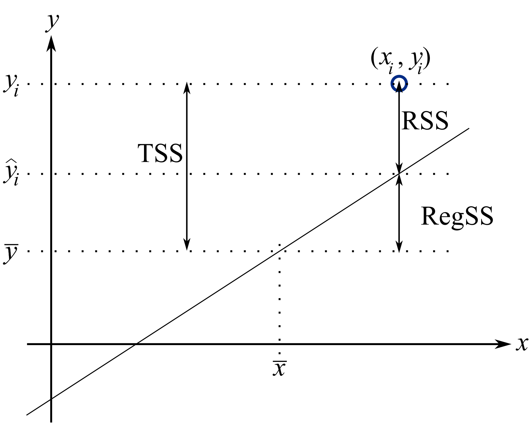
The total sum of squares (TSS) is the total variance in the vector of \(y\)-data. This broken down into two components: the sum of squares due to regression, \(\sum \left(\hat{y}_i - \overline{y}\right)^2\), called RegSS, and the sum of squares of the residuals (RSS), \(\sum e_i^2 = e^T e\).
It is convenient to write these sums of squares (variances) in table form, called an Analysis of Variance (ANOVA) table:
Type of variance
Distance
Degrees of freedom
SSQ
Mean square
Regression
\(\hat{y}_i - \overline{y}\)
\(k-1\) (\(k=2\) in the examples so far)
RegSS
\(\text{RegSS}/(k-1)\)
Error
\(y_i - \hat{y}_i\)
\(n-k\)
RSS
\(\text{RSS}/(n-k)\)
Total
\(y_i - \overline{y}\)
\(n-1\)
TSS
\(\text{TSS}/(n-1)\)
Here \(k\) is the number of parameters estimated in the model, so \(k = 2\) for the model \(\hat{y}_i = b_0 + b_1 x_i\). The degrees of freedom follow from the distances in the second column. The total row uses \(n-1\), not \(n\), because the \(n\) distances \(y_i - \overline{y}\) are computed from the estimated mean \(\overline{y}\), which removes one degree of freedom (seen earlier when estimating a variance). The error row uses \(n-k\), since \(k\) parameters were estimated to compute the \(\hat{y}_i\). The regression row gets the difference, \((n-1) - (n-k) = k-1\), which is the number of predictor terms in the model (one, for a straight line). The degrees of freedom of the regression and error rows add up to the total row, as do the sums of squares.
The ratio of the two mean squares in the last column is called the \(F\)-statistic:
It compares the variance explained by the model against the variance left in the residuals. A value of \(F_0\) near 1.0 says the model explains about as much per degree of freedom as the noise; a large \(F_0\) says the model explains far more than could be expected from noise. Software packages report this number, together with the two degrees of freedom used to compute it, and a p-value; we will point it out in the software output later in this section.
4.7.1.1. Interpreting the standard error
The term \(S_E^2 = \text{RSS}/(n-k)\) is one way of quantifying the model’s performance. The value \(S_E = \sqrt{\text{RSS}/(n-k)} = \sqrt{(e^Te)/(n-k)}\) is called the standard error. It is really just the standard deviation of the error term, accounting correctly for the degrees of freedom. It carries the units of the \(\mathrm{y}\)-variable, so it can be compared directly against the accuracy that the application requires.
Example: Assume we have a model for predicting batch yield in kilograms from \(\mathrm{x}\) = raw material purity, what does a standard error of 3.4 kg imply?
Answer: Recall if the assumption of normally distributed errors is correct, then this value of 3.4 kg indicates that about two thirds of the yield prediction errors will lie within \(\pm 3.4\) kg, and that 95% of the prediction errors will lie within \(\pm 2 \times 3.4\) kg. We will quantify the prediction interval more precisely, but the standard error is a good approximation for the error of \(\mathrm{y}\).
4.7.1.2. Exercise
For two extreme cases:
\(y_i = e_i\), i.e. where \(b_0 = 0\) and \(b_1 = 0\). In other words, our \(y_i\) measurements are just random noise.
\(y_i = b_0 + b_1 x_i + e_i\), for any values of \(b_0\) and \(b_1\), that model fits the data perfectly, with no residuals.
Do the following in the space below:
draw a generic plot
create an ANOVA table with fake values
write down the value of the ratio \(\dfrac{\text{RegSS}}{\text{TSS}}\)
also write down what happens to \(F_0 = \dfrac{\text{RegSS}/(k-1)}{\text{RSS}/(n-k)}\), the ratio of the two mean squares, in each case
From this exercise we learn that:
The null model (\(y_i = e_i\)) has ratio \(\dfrac{\text{RegSS}}{\text{TSS}} = 0\).
Models where the fit is perfect have a ratio \(\dfrac{\text{RegSS}}{\text{TSS}} = 1\). This number is called \(R^2\), and we will see why it is called that next.
4.7.1.3. Derivation of \(R^2\)
As introduced by example in the previous part, \(R^2 = \dfrac{\text{RegSS}}{\text{TSS}} = \dfrac{\sum_i{ \left(\hat{y}_i - \overline{\mathrm{y}}\right)^2}}{\sum_i{ \left(y_i - \overline{\mathrm{y}}\right)^2}}\): simply the ratio between the variance we can explain with the model (RegSS) and the total variance we started off with (TSS). We can also write that \(R^2 = 1-\dfrac{\text{RSS}}{\text{TSS}}\), based on the fact that TSS = RegSS + RSS.
From the above ratios it is straightforward to see that if \(R^2 = 0\), it requires that \(\hat{y}_i = \overline{\mathrm{y}}\): we are predicting just a flat line, the mean of the \(\mathrm{y}\) data. On the other extreme, an \(R^2 = 1\) implies that \(\hat{y}_i = y_i\), we have perfect predictions for every data point.
The nomenclature \(R^2\) comes from the fact that, for a model with a single \(\mathrm{x}\)-variable, it is the square of the correlation between \(\mathrm{x}\) and \(\mathrm{y}\). (In the general case, with several \(\mathrm{x}\)-variables, \(R^2\) is the square of the correlation between \(\mathrm{y}\) and \(\hat{y}\).) Recall from the correlation section that
and can range in value from \(-1\) to \(+1\). The \(R^2\) ranges from 0 to +1, and is the square of \(r(x,y)\). \(R^2\) is just a way to tell how far we are between predicting a flat line (no variation) and the extreme of being able to predict the model building data, \(y_i\), exactly.
The \(R^2\) value is likely well known to anyone that has encountered least squares before. It is most widely used as an answer to the question “how good is my model”. You have likely said or heard something like this before:
“the \(R^2\) value is really high, 90%, so this is a good model”.
“Wow, that’s a really low \(R^2\), this model can’t be right - it’s no good”.
The next two subsections take that question apart: first what the \(R^2\) value is measuring, and then which quantity answers the question you actually had in mind.
4.7.1.4. Two properties of \(R^2\)
Two properties of \(R^2\) mark out what it can and cannot report on. Both are for the straight-line model with an intercept, \(\hat{y}_i = b_0 + b_1 x_i\), fitted by least squares.
The value is unchanged when the roles of the two variables are swapped. Both the numerator and the denominator of \(r(x,y)\) are symmetric in the two variables, so regressing \(\mathrm{y}\) on \(\mathrm{x}\) and regressing \(\mathrm{x}\) on \(\mathrm{y}\) return the same \(R^2\), even though the two models have different slopes and intercepts. Using the 11-point example from this section:
Python, 17 lines
import numpy as np
import statsmodels.api as sm

x = np.array([10, 8, 13, 9, 11, 14, 6, 4, 12, 7, 5])
y = np.array([8.04, 6.95, 7.58, 8.81, 8.33, 9.96,
              7.24, 4.26, 10.84, 4.82, 5.68])

# Predict y from x, then x from y:
forward = sm.OLS(y, sm.add_constant(x)).fit()
reverse = sm.OLS(x, sm.add_constant(y)).fit()

# Both print 0.6665, though the slopes are
# 0.5001 and 1.3328 respectively:
print(f"{forward.rsquared:.4f}  {reverse.rsquared:.4f}")

# And the same value again, with no model fitted:
print(f"{np.corrcoef(x, y)[0, 1] ** 2:.4f}")
Drawing both lines on the same axes, in the figure below, shows what the two models are doing differently. Each minimizes a different set of distances: vertical distances to the line when predicting \(\mathrm{y}\) from \(\mathrm{x}\), and horizontal distances when predicting \(\mathrm{x}\) from \(\mathrm{y}\). Both lines pass through \((\overline{x}, \overline{y})\), and both report \(R^2 = 0.6665\).
Python, 43 lines
import plotly.graph_objects as go

b0, b1 = forward.params
a0, a1 = reverse.params
grid = np.linspace(2.5, 15.5, 200)

# The distances each model minimizes. The `None`
# entries break the trace between the segments.
vertical_x, vertical_y = [], []
horizontal_x, horizontal_y = [], []
for xi, yi in zip(x, y):
    vertical_x += [xi, xi, None]
    vertical_y += [yi, b0 + b1 * xi, None]
    horizontal_x += [xi, a0 + a1 * yi, None]
    horizontal_y += [yi, yi, None]

fig = go.Figure()
fig.add_scatter(x=vertical_x, y=vertical_y, mode="lines",
                line=dict(color="#0072B2", width=1),
                showlegend=False)
fig.add_scatter(x=horizontal_x, y=horizontal_y, mode="lines",
                line=dict(color="#D55E00", width=1),
                showlegend=False)
fig.add_scatter(x=grid, y=b0 + b1 * grid, mode="lines",
                line=dict(color="#0072B2", width=3),
                name=f"Predicting y from x: slope {b1:.3f}")

# The reverse model, x = a0 + a1 * y, rewritten as a
# line in these (x, y) axes:
fig.add_scatter(x=grid, y=(-a0 / a1) + (1 / a1) * grid,
                mode="lines",
                line=dict(color="#D55E00", width=3, dash="dash"),
                name=f"Predicting x from y: slope "
                     f"{1 / a1:.3f} in these axes")
fig.add_scatter(x=x, y=y, mode="markers", name="Data",
                marker=dict(color="black", size=9))
fig.add_scatter(x=[x.mean()], y=[y.mean()], mode="markers",
                name="Mean of the data",
                marker=dict(color="#666666", size=14,
                            symbol="cross"))
fig.update_layout(xaxis_title="x", yaxis_title="y",
                  width=900, height=600)
fig.show()

The 11-point example with both least squares lines drawn. The solid line predicts \(\mathrm{y}\) from \(\mathrm{x}\) and minimizes the vertical distances; the dashed line predicts \(\mathrm{x}\) from \(\mathrm{y}\) and minimizes the horizontal ones. The slopes are 0.500 and 0.750 (the second rewritten in these axes), and both models report \(R^2 = 0.6665\).
The value can be calculated before the model is fitted. The last line of that code shows it: \(R^2 = r(x,y)^2\), and the correlation is computed from the raw data columns alone. It does not require the slope, the intercept, or the residuals. This is not a coincidence of these particular numbers; it is what \(r(x,y)\), and therefore \(R^2\), is defined to measure: the strength of the linear association between two sequences of numbers.
Two boundaries on that second property are worth stating:
With more than one \(\mathrm{x}\)-variable, \(R^2\) is the square of the correlation between \(\mathrm{y}\) and \(\hat{y}\), so the model does have to be fitted first.
The two expressions \(\text{RegSS}/\text{TSS}\) and \(1 - \text{RSS}/\text{TSS}\) agree only for a least squares fit with an intercept, evaluated on the same data used to fit it. Applied to new data the second expression is the one that is reported, and it can fall below zero: that happens when the model’s predictions on the new data have larger squared errors than simply using \(\overline{y}\) of the new data.
A third property, that \(R^2\) on the building data cannot decrease when a term is added to the model, is shown in the MLR section. It is the reason the adjusted R-squared is sometimes reported instead, dividing each sum of squares by its degrees of freedom:
where \(k=2\) for the case of estimating a model \(y_i = b_0 + b_1 x_i\), as there are 2 parameters.
4.7.1.5. Matching the metric to the purpose of the model
There are two common reasons for building a linear model, and each has a metric that reports on it directly:
To learn about the system, by interpreting the slope or the intercept. Here the confidence interval for that coefficient is the matching quantity. A reaction rate reported as \(k = 0.81 \pm 0.26\,\text{s}^{-1}\) and the same rate reported as \(k = 0.81 \pm 0.68\,\text{s}^{-1}\) support quite different conclusions, and the interval is in units of \(\text{s}^{-1}\), which is what the reactor design calculation requires.
To predict a new \(y\) value. Here the matching quantities are the standard error, \(S_E\), and the prediction interval. Both are in the units of \(\mathrm{y}\): a prediction interval states the range, in kilograms or kPa, in which the next observation is expected to fall, and an \(R^2\) of 0.78 does not.
The \(S_E\) calculated on the building data is a within-sample number. The standard deviation of the residuals on testing data, or from cross-validation when no testing data can be set aside, is the same quantity computed on observations the model has not seen.
A higher \(R^2\) does correspond to a narrower confidence interval and a smaller standard error, and for the single-\(\mathrm{x}\) model the connection is exact. Writing \(z = b_1 / S_E(b_1)\) for the ratio reported in the software output, and \(s_y\) for the standard deviation of the \(y\)-data:
where \(k = 2\) for the straight-line model, so \(n-k = 9\) in the example below.
Both relationships are relative. The first fixes the width of the slope’s confidence interval as a fraction of the slope itself: at \(R^2 = 0.6665\) and \(n = 11\) we get \(z = 4.24\), and with \(c_t = 2.26\) the interval half-width is \(c_t/z = 53\%\) of \(b_1\), matching the \(0.233 \leq \beta_1 \leq 0.767\) interval calculated in the subsection on confidence intervals for the coefficients below. The second fixes \(S_E\) as a fraction of the spread of the \(\mathrm{y}\)-data: the same \(R^2\) gives a standard error of 0.3 kPa on data with \(s_y = 0.5\) kPa, and 3 kPa on data with \(s_y = 5\) kPa. That is why no threshold on \(R^2\), agreed ahead of time, can tell you whether a model is adequate: what counts as an acceptable \(S_E\) is set by the application, not by the variance ratio.
The distillation tower model built later in this section gives a worked instance: \(R^2 = 0.781\) with \(s_y = 6.25\) kPa produces \(S_E = 2.94\) kPa. Whether a spread of roughly \(\pm 6\) kPa on a predicted vapour pressure is usable is a question about the process, and the 0.781 by itself does not answer it.
One further point about the range of the data: \(R^2\) depends on how widely the \(\mathrm{x}\)-values were sampled. Collect data over a narrow band of \(\mathrm{x}\), and the TSS shrinks while the residual variance stays where it is, so \(R^2\) drops even though the underlying relationship, the slope, and \(S_E\) are unchanged. Two \(R^2\) values from different data sets are therefore not comparable, while two \(S_E\) values, in the units of \(\mathrm{y}\), are.
Both effects can be shown together by simulating from a single model, \(y = 5 + 1.0 x + e\), and changing only two things: the size of the error, and how widely \(\mathrm{x}\) was sampled. In the four panels below, \(R^2\) runs from 0.60 to 0.97 while the relationship being estimated never changes.
Python, 55 lines
from plotly.subplots import make_subplots

rng = np.random.default_rng(225)
n_sim = 40

# The full range of x, then its middle half:
spreads = {
    "x sampled over 0 to 20": (0.0, 20.0),
    "x sampled over 5 to 15": (5.0, 15.0),
}

fig = make_subplots(
    rows=2, cols=2, shared_xaxes=True, shared_yaxes=True,
    subplot_titles=list(spreads) + ["", ""],
)
for row, target in enumerate([1.0, 2.0], start=1):
    for col, (low, high) in enumerate(spreads.values(), start=1):
        x_sim = rng.uniform(low, high, n_sim)
        errors = rng.normal(0.0, 1.0, n_sim)

        # Rescale the errors so that the realised
        # standard error is exactly the target. The
        # residuals are linear in the errors, so
        # scaling the errors scales S_E to match.
        X_sim = sm.add_constant(x_sim)
        draw = sm.OLS(5.0 + x_sim + errors, X_sim).fit()
        y_sim = (5.0 + 1.0 * x_sim
                 + errors * target / np.sqrt(draw.scale))

        sim = sm.OLS(y_sim, X_sim).fit()
        se_sim = np.sqrt(sim.scale)
        grid_sim = np.linspace(low, high, 100)

        fig.add_scatter(x=x_sim, y=y_sim, mode="markers",
                        marker=dict(color="#0072B2"),
                        row=row, col=col, showlegend=False)
        fig.add_scatter(
            x=grid_sim,
            y=sim.predict(sm.add_constant(grid_sim)),
            mode="lines", line=dict(color="#D55E00", width=3),
            row=row, col=col, showlegend=False,
        )
        fig.add_annotation(
            text=f"R<sup>2</sup> = {sim.rsquared:.2f}<br>"
                 f"S<sub>E</sub> = {se_sim:.1f} kg<br>"
                 f"slope = {sim.params[1]:.2f} kg/unit",
            xref="x domain", yref="y domain",
            x=0.04, y=0.96, align="left", showarrow=False,
            row=row, col=col,
        )

fig.update_xaxes(title_text="x", row=2)
fig.update_yaxes(title_text="y [kg]", col=1)
fig.update_layout(width=1000, height=780)
fig.show()

Four data sets simulated from \(y = 5 + 1.0 x + e\). The errors are scaled so that the realised standard error is exactly 1.0 kg in the top row and exactly 2.0 kg in the bottom row, and the two shaded panels report the same \(R^2\) of 0.90.
There are three comparisons to make in the figure:
Along a row, the prediction error is identical in the two panels while \(R^2\) changes: 0.97 and 0.90 in the top row, 0.90 and 0.60 in the bottom row. The panels differ only in the range of \(\mathrm{x}\) that was sampled, so \(R^2\) has moved with no change in how accurately either model predicts.
Down a column, the range of \(\mathrm{x}\) is held the same and the size of the error is what differs: doubling the error takes \(R^2\) from 0.97 to 0.90 on the left, and from 0.90 to 0.60 on the right. This is the comparison in which \(R^2\) moves for the reason usually attached to it.
Across the two shaded panels, \(R^2\) is 0.90 in both, and the prediction error in one is twice that in the other: \(S_E\) = 1.0 kg against 2.0 kg.
The slope is recovered in all four panels, between 0.97 and 1.00 kg per unit of \(\mathrm{x}\). The quantity to report when the purpose is to learn about the system is unaffected by either change.
Both of the first two comparisons follow from what the ratio contains. \(R^2\) is the share of the variation in \(\mathrm{y}\) that the model accounts for, and the variation in \(\mathrm{y}\) grows as the \(\mathrm{x}\)-values are spread further apart. There are then two ways to raise it: reduce the error, or sample \(\mathrm{x}\) over a wider range. Only the first changes what the model can predict. Read this way, \(R^2\) reports whether the range of \(\mathrm{x}\) was wide enough for the trend to stand out against the error, which is a question about how the data were collected, rather than reporting how large the prediction error is.
The standard error is not open to that second reading. It is in kilograms here, and it stays at 1.0 kg or 2.0 kg whether \(\mathrm{x}\) was sampled over the full range or over the middle half of it, which is what makes it comparable between two data sets.
Two consequences follow for practical work. A model built on data from a narrow operating window will report a low \(R^2\) even when the measurements are precise, which is a common situation with routine process data. Widening the range covered by an experiment raises \(R^2\) on its own, with no change in the prediction error.
This leaves \(R^2\) with a clear and narrower reading: it reports how strongly \(\mathrm{x}\) and \(\mathrm{y}\) are linearly associated, on the data in hand. That is a useful thing to know, and it is a different question from either of the two purposes listed at the start of this subsection. The suitability of a model for a particular purpose is better assessed by:
your engineering judgment: does the interpretation of model parameters make sense?
the confidence intervals for the coefficients, the standard error and the prediction interval,
testing data, or cross-validation tools (we will see this topic later on), to see how well the model performs on new, unseen and unused observations.
4.7.2. Confidence intervals for the model coefficients \(b_0\) and \(b_1\)
Note
A good reference for this section is the book by Fox (Chapter 6), and the book by Draper and Smith.
Up to this point we have made no assumptions about the data. In fact we can calculate the model estimates, \(b_0\) and \(b_1\) as well as predictions from the model without any assumptions on the data. It is only when we need additional information such as confidence intervals for the coefficients and prediction error estimates that we must make assumptions.
Recall the \(b_1\) coefficient represents the average change in \(\mathrm{y}\) associated with a 1-unit change in the \(\mathrm{x}\)-variable. Let’s say you are estimating a reaction rate (kinetics) from a linear least squares model, a standard step in reactor design, you would want a measure of confidence of your coefficient. For example, if you calculate the reaction rate as \(k = b_1 = 0.81 \,\text{s}^{-1}\) you would benefit from knowing whether the 95% confidence interval was \(k = 0.81 \pm 0.26 \,\text{s}^{-1}\) or \(k = 0.81 \pm 0.68 \,\text{s}^{-1}\). In the latter case it is doubtful whether the reaction rate is of practical significance. Point estimates of the least squares model parameters are satisfactory, but the confidence interval information is richer to interpret.
We first take a look at some assumptions in least squares modelling, then return to deriving the confidence interval.
4.7.2.1. Assumptions required for analysis of the least squares model
Recall that the population (true) model is \(y_i = \beta_0 + \beta_1 x_i + \epsilon_i\) and \(b_0\) and \(b_1\) are our estimates of the model’s coefficients, and \(\mathrm{e}\) be the estimate of the true error \(\epsilon\). Note we are assuming imperfect knowledge of the \(y_i\) by lumping all errors into \(e_i\). For example, measurement error, structural error (we are not sure the process follows a linear structure), inherent randomness, and so on.
Furthermore, our derivation for the confidence intervals of \(b_0\) and \(b_1\) requires that we assume:
Linearity of the model, and that the values of \(\mathrm{x}\) are fixed (have no error). This implies that the error captured by \(\epsilon\) is the error of \(\mathrm{y}\), since the \(\beta_0 + \beta_1 \mathrm{x}\) terms are fixed.
In an engineering situation this would mean that your \(\mathrm{x}\) variable has much less uncertainty than the \(\mathrm{y}\) variable; and is often true in many situations.
The variance of \(\mathrm{y}\) is the same (constant) at all values of \(\mathrm{x}\), known as the constant error variance assumption.
The variability of \(\mathrm{y}\) can be non-constant in several practical cases (e.g. our measurement accuracy deteriorates at extreme high and low levels of \(\mathrm{x}\)).
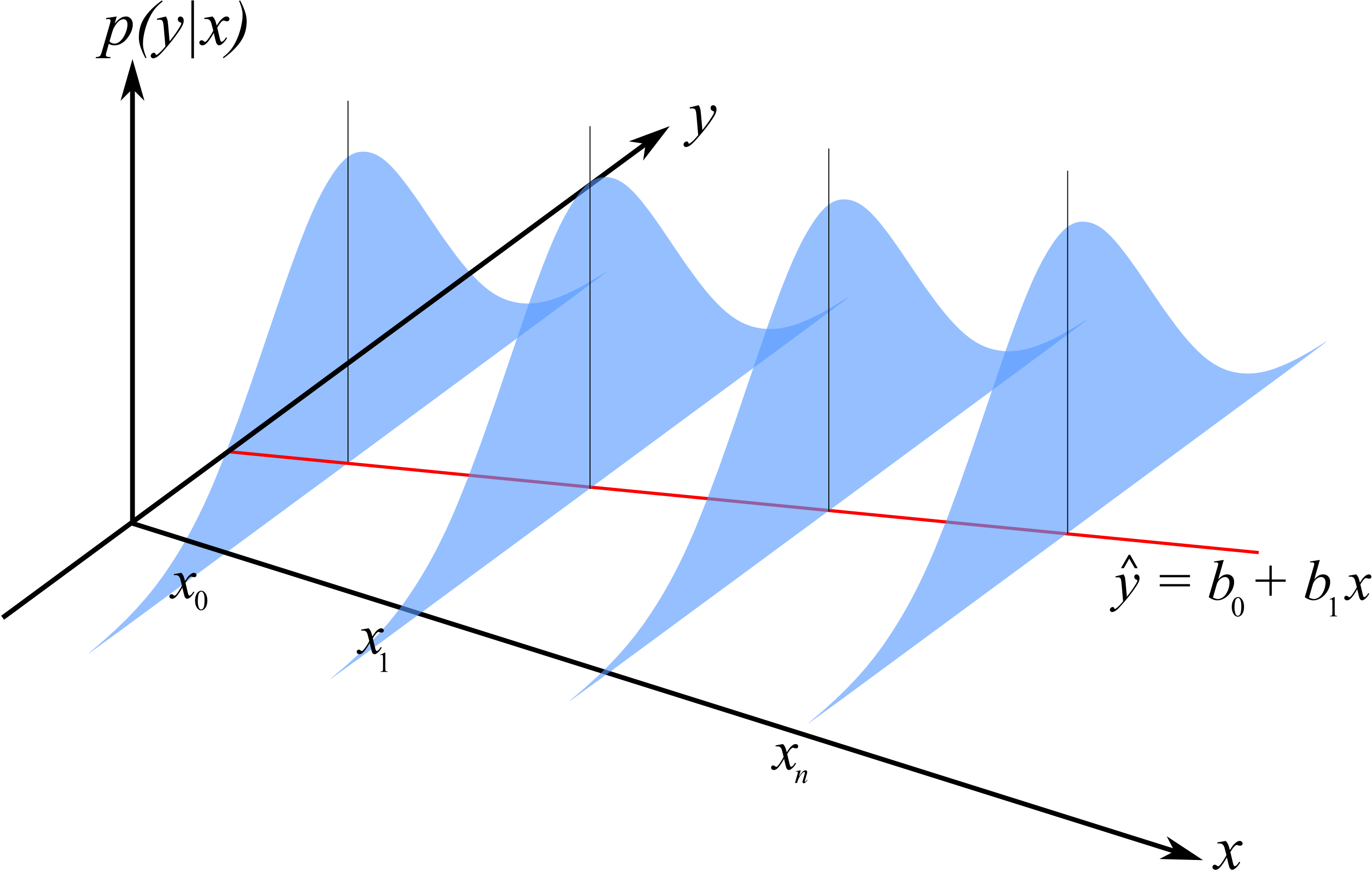
Illustration of the constant error variance assumption and the normally distributed error assumption.
The errors are normally distributed: \(\epsilon_i \sim \mathcal{N}(0, \sigma_\epsilon^2)\). This also implies that \(y_i \sim \mathcal{N}(\beta_0 + \beta_1x_i, \sigma_\epsilon^2)\) from the first linearity assumption. (The residuals \(e_i\) are our estimates of the unobservable \(\epsilon_i\), so this assumption is checked by examining the residuals.)
Each error is independent of the other. This assumption is often violated in cases where the observations are taken in time order on slow moving processes (e.g. if you have a positive error now, your next sample is also likely to have a positive error). We will have more to say about this later when we check for independence with an autocorrelation test.
In addition to the fact that the \(\mathrm{x}\) values are fixed, we also assume they are independent of the error. If the \(\mathrm{x}\) value is fixed (i.e. measured without error), then it is already independent of the error.
When the \(\mathrm{x}\) values are not fixed, there are cases where the error gets larger as \(\mathrm{x}\) gets smaller/larger.
All \(y_i\) values are independent of each other. This again is violated in cases where the data are collected in time order and the \(y_i\) values are autocorrelated.
Note
Derivation of the model’s coefficients do not require these assumptions, only the derivation of the coefficient’s confidence intervals require this.
Also, if we want to interpret the model’s \(S_E\) as the estimated standard deviation of the residuals, then it helps if the residuals are normally distributed.
4.7.2.2. Confidence intervals for \(\beta_0\) and \(\beta_1\)
Recall from our discussions on confidence intervals that we need to know the mean and variance of the population from which \(b_0\) and \(b_1\) come. Note that \(\beta_0\) and \(\beta_1\) are fixed population values; it is our estimates \(b_0\) and \(b_1\) that vary from one data sample to the next, and so have a distribution. Specifically for the least squares case:
Once we know those parameters, we can create a \(z\)-value for \(b_0\) and \(b_1\), and then calculate the confidence interval for \(\beta_0\) and \(\beta_1\). So our quest now is to calculate \(\mathcal{V}\{b_0\}\) and \(\mathcal{V}\{b_1\}\), and we will use the 6 assumptions we made in the previous part.
Start from the equations that define \(b_0\) and \(b_1\) in the prior section where we showed that:
In going from the second line to the third, the \(\overline{\mathrm{y}}\) term drops out. Expand the numerator: \(\sum_i \left(x_i - \overline{\mathrm{x}}\right)\left(y_i - \overline{\mathrm{y}}\right) = \sum_i \left(x_i - \overline{\mathrm{x}}\right)y_i - \overline{\mathrm{y}} \sum_i \left(x_i - \overline{\mathrm{x}}\right)\), and the last sum is zero, since \(\sum_i \left(x_i - \overline{\mathrm{x}}\right) = 0\) by the definition of the mean. So \(\overline{\mathrm{y}}\) is the average of all the \(y_i\), but here it multiplies a quantity that is identically zero, so it has no effect on \(b_1\).
That last form of expressing \(b_1\) shows that every data point contributes a small amount to the coefficient \(b_1\). But notice how it is broken into 2 pieces: each term in the sum has a component due to \(m_i\) and one due to \(y_i\). The \(m_i\) term is a function of the x-data only, and since we assume the x’s are measured without error, that term has no error. The \(y_i\) component is the only part that has error.
Up to this point \(b_1\) is a single number, computed from the data in hand. To describe how precise that number is, we change how we read the \(y_i\). We now treat each \(y_i\) as one realisation of a random variable, drawn from \(y_i \sim \mathcal{N}(\beta_0 + \beta_1 x_i, \sigma_\epsilon^2)\) (assumptions 1 to 3). Imagine repeating the experiment: hold every \(x_i\) at exactly the same setting, take a fresh measurement of each \(y_i\), and recompute \(b_1\). Each repeat gives a slightly different \(b_1\). The expectation \(\mathcal{E}\{b_1\}\) and variance \(\mathcal{V}\{b_1\}\) below describe the distribution of \(b_1\) over those hypothetical repeats. Because the \(x_i\) are held fixed, the weights \(m_i\) are constants that carry no error, and the only randomness enters through the \(y_i\).
So we can write:
where \(j\) is an index for all data points used to build the least squares model.
Two rules take us from the expectation line to the variance line. First, a constant multiplying a random variable comes out of the variance as its square, \(\mathcal{V}\{m_i y_i\} = m_i^2 \mathcal{V}\{y_i\}\), in the same way that \(\mathcal{E}\{m_i y_i\} = m_i \mathcal{E}\{y_i\}\) for the expectation. Second, the variance of a sum equals the sum of the individual variances only when the terms are independent. That is assumption 6, that the \(y_i\) are independent of one another; the cross-covariance terms are then zero, so no products between different \(y_i\) appear. If the \(y_i\) were correlated, for example data collected in time order, those cross terms would not vanish and this step would not hold.
The last two lines use assumption 2, the constant error variance: every \(\mathcal{V}\{y_i\}\) has the same value, so it factors out of the sum to leave \(\mathcal{V}\{b_1\} = \mathcal{V}\{y_i\} \sum_i m_i^2\). The remaining sum collapses because \(\sum_i m_i^2 = \dfrac{\sum_i (x_i - \overline{\mathrm{x}})^2}{\left(\sum_j (x_j - \overline{\mathrm{x}})^2\right)^2} = \dfrac{1}{\sum_j (x_j - \overline{\mathrm{x}})^2}\).
Questions:
So now apart from the numerator term, how could you decrease the error in your model’s \(b_1\) coefficient?
Use samples that are far from the mean of the \(\mathrm{x}\)-data.
Use more samples.
What do we use for the numerator term \(\mathcal{V}\{y_i\}\)?
This term represents the variance of the \(y_i\) values at a given point \(x_i\). It is the variance of \(y_i\) about its true value on the line (the error variance), not the spread of the \(y_i\) about their overall average \(\overline{\mathrm{y}}\). If you took repeated measurements at a fixed \(x_i\), it is the variance you would see around the average of those repeats; with no replicates we estimate it by pooling the residuals about the fitted line. If (a) there is no evidence of lack-of-fit (which can be tested formally when the design has replicated points), and (b) if \(\mathrm{y}\) has the same error at all levels of \(\mathrm{x}\), then we can write that \(\mathcal{V}\{y_i\}\) = \(\mathcal{V}\{e_i\} = \dfrac{\sum{e_i^2}}{n-k}\), where \(n\) is the number of data points used, and \(k\) is the number of coefficients estimated (2 in this case). The \(n-k\) quantity is the degrees of freedom.
Now for the variance of \(b_0 = \overline{\mathrm{y}} - b_1 \overline{\mathrm{x}}\). The only terms with error are \(b_1\), and \(\overline{\mathrm{y}}\). So we can derive that:
Summary of important equations
For convenience we will define some short-hand notation, which is common in least squares:
You will see that \(S_E\) is an estimate of the standard deviation of the error (residuals), while \(S_E(b_0)\) and \(S_E(b_1)\) are the standard deviations of estimates for \(b_0\) and \(b_1\) respectively.
Now it is straight forward to construct confidence intervals for the least squares model parameters. You will also realize that we have to use the \(t\)-distribution, because we are using an estimate of the variance.
Example
Returning back to our ongoing example, we can calculate the confidence interval for \(\beta_0\) and \(\beta_1\). We calculated earlier already that \(b_0\) = 3.0 and \(b_1\) = 0.5. Using these values we can calculate the standard error:
Python, 34 lines
import numpy as np
import statsmodels.api as sm

x = np.array([10, 8, 13, 9, 11, 14, 6, 4, 12, 7, 5])
y = np.array([8.04, 6.95, 7.58, 8.81, 8.33, 9.96,
              7.24, 4.26, 10.84, 4.82, 5.68])

# Calculate the linear model, where y
# is described by x.
X = sm.add_constant(x)
mod_ls = sm.OLS(y, X).fit()

# We can find what `b0` and `b1` are in
# several different ways:
print(mod_ls.summary())

# or using
print("The model coefficients are: ")
mod_ls.params

# Model predictions:
print("The predicted values are: ")
mod_ls.predict()
# [ 8.001  7.000  9.501  7.501  8.501
#  10.001  6.000  5.000  9.001  6.500  5.501]

# Prediction error = observed - predicted
error = y - mod_ls.predict()
N = len(x)

# The SE = standard error = 1.236603
std_error = np.sqrt((error ** 2).sum() / (N - 2))
print(f"Standard error SE = "
      f"{round(std_error, 3)}")
R, 30 lines
x <- c(10, 8, 13, 9, 11, 14, 6, 4, 12, 7, 5)
y <- c(8.04, 6.95, 7.58, 8.81, 8.33, 9.96,
      7.24, 4.26, 10.84, 4.82, 5.68)

# "Calculate for me the linear model,
# where y is described by x"
mod.ls <- lm(y ~ x)

# We can find what the "b0" and "b1"
# values are in several different ways:
summary(mod.ls)

# or using
print('The model coefficients are: ')
coefficients(mod.ls)

# Model predictions:
print('The predicted values are: ')
predict(mod.ls)
# 8.001  7.000  9.501  7.501  8.501
# 10.001  6.00  5.000  9.001  6.500  5.501

# Prediction error = observed - predicted
error <- y - predict(mod.ls)
N <- length(x)

# The SE = standard error = 1.236603
std.error <- sqrt(sum(error^2) / (N-2))
paste0('Standard error SE = ',
       round(std.error, 3))
Use that \(S_E\) value to calculate the confidence intervals for \(\beta_0\) and \(\beta_1\), and use that \(c_t = 2.26\) at the 95% confidence level. You can calculate this value in R using qt(0.975, df=(N-2)). There are \(n-2\) degrees of freedom, the number of degrees of freedom used to calculate \(S_E\).
First calculate the \(S_E\) value and the standard errors for the \(b_0\) and \(b_1\). Substitute these into the equation for the confidence interval and calculate:
The 95% confidence interval for \(\beta_0\):
The confidence interval for \(\beta_1\):
The plot shows the effect of varying the slope parameter, \(b_1\), from its lower bound to its upper bound. Notice that the slope always passes through the mean of the data \((\overline{x}, \overline{y})\).
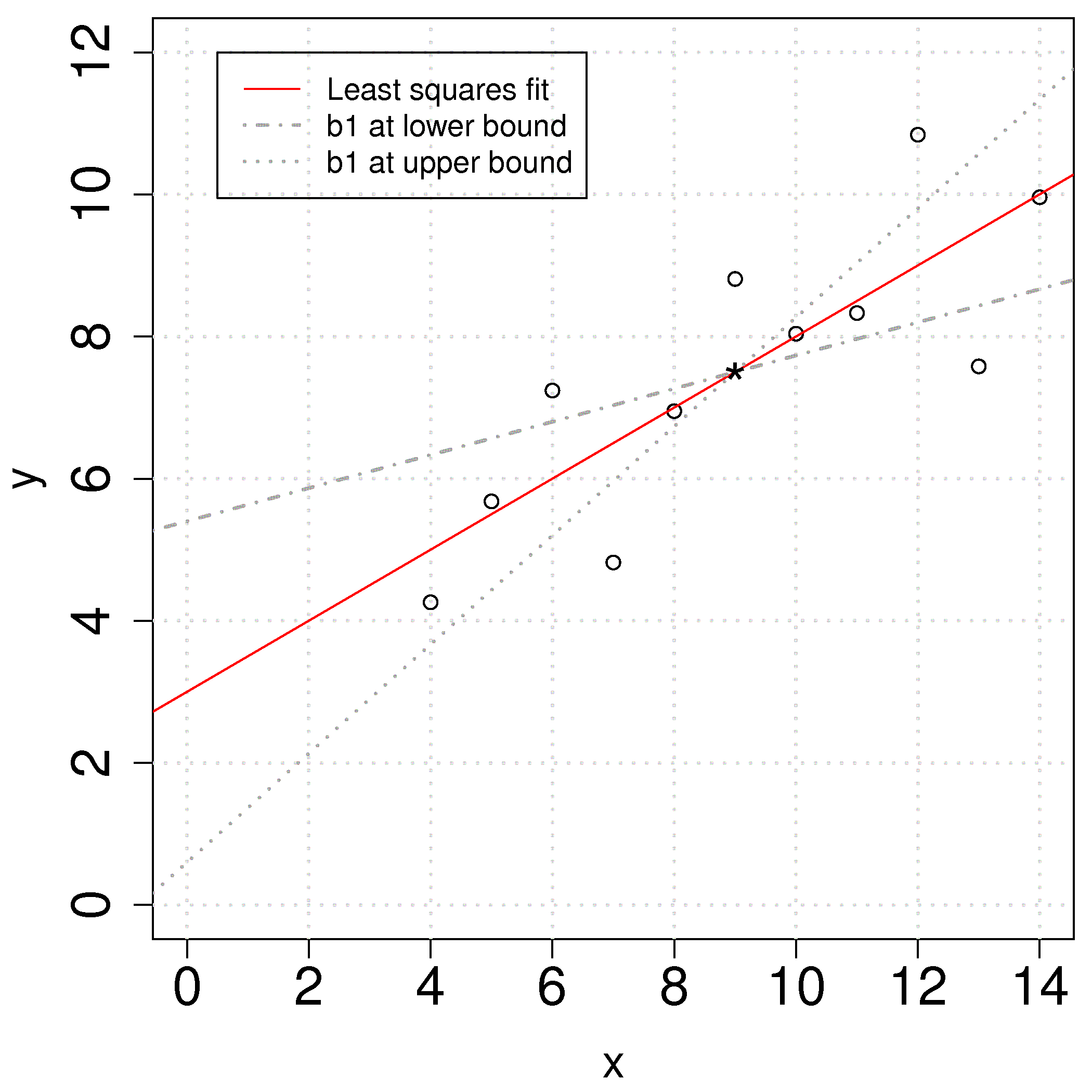
In many cases the confidence interval for the intercept is not of any value because the data for \(\mathrm{x}\) is so far away from zero, or the true value of the intercept is not of concern for us.
Python, 32 lines
import numpy as np
import statsmodels.api as sm

x = np.array([10, 8, 13, 9, 11, 14, 6, 4, 12, 7, 5])
y = np.array([8.04, 6.95, 7.58, 8.81, 8.33, 9.96,
              7.24, 4.26, 10.84, 4.82, 5.68])

# Calculate the linear model, where y
# is described by x.
X = sm.add_constant(x)
mod_ls = sm.OLS(y, X).fit()

# You can (and should at the beginning)
# calculate the confidence intervals as shown
# above. But there is a short-cut, to save
# time, and is less error prone:
mod_ls.conf_int()

#                  0         1
# const     0.455737  5.544445
# x1        0.233370  0.766812

# If you want the confidence interval at any
# other level, for example, at the 90% level:
mod_ls.conf_int(alpha=0.10)

#                  0         1
# const     0.938303  5.061879
# x1        0.283957  0.716225

# Compare this to the calculated value by hand
# above. It is exactly the same!
R, 28 lines
x <- c(10, 8, 13, 9, 11, 14, 6, 4, 12, 7, 5)
y <- c(8.04, 6.95, 7.58, 8.81, 8.33, 9.96,
      7.24, 4.26, 10.84, 4.82, 5.68)

# "Calculate for me the linear model,
# where y is described by x"
mod.ls <- lm(y ~ x)

# You can (and should at the beginning)
# calculate the confidence intervals as shown
# above. But there is a short-cut, to save
# time, and is less error prone:
confint(mod.ls)

#                 2.5 %    97.5 %
# (Intercept) 0.4557369 5.5444449
# x           0.2333701 0.7668117

# If you want the confidence interval at any
# other level, for example, at the 90% level:
confint(mod.ls, level=0.90)

#                   5 %     95 %
# (Intercept) 0.9383030 5.061879
# x           0.2839568 0.716225

# Compare this to the calculated value by hand
# above. It is exactly the same!
4.7.3. Prediction error estimates for the y-variable
Apart from understanding the error in the model’s coefficient, we also would like an estimate of the error when predicting \(\hat{y}_i\) from the model, \(y_i = b_0 + b_1 x_i + e_i\) for a new value of \(x_i\). This is known as the prediction interval, or prediction error interval.
4.7.3.1. A naive first attempt
We might expect the error is related to the average size of the residuals. After all, our assumptions we made earlier showed the standard error of the residuals was the standard error of the \(\mathrm{y}\): \(S_E^2 = \mathcal{V}\left\{e_i\right\} = \mathcal{V}\left\{y_i\right\} = \dfrac{\sum{e_i^2}}{n-k}\).
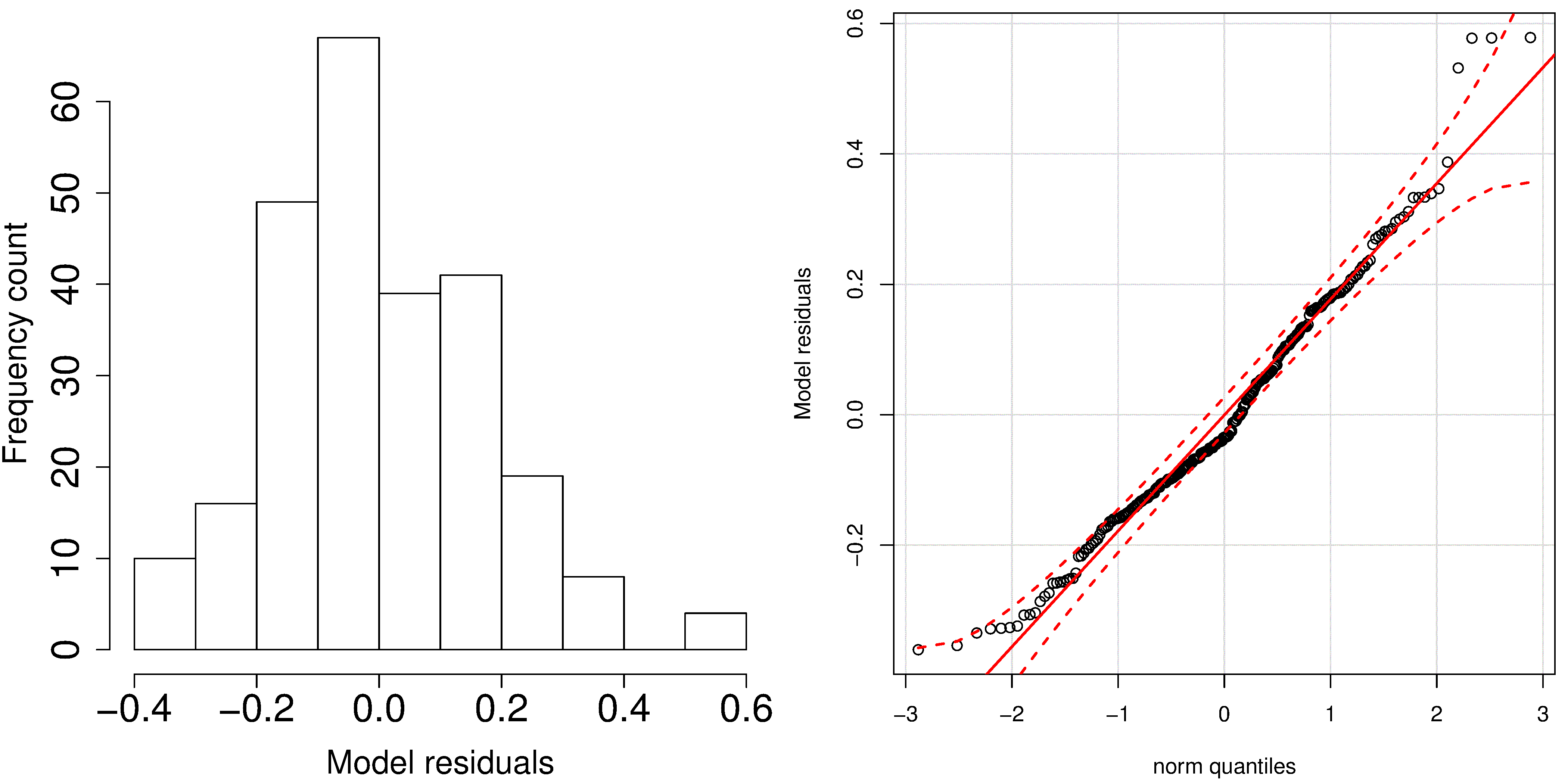
A typical histogram of the residuals looks as shown here: it is always centered around zero, and appears to be normally distributed. So we could expect to write our prediction error as \(\hat{y}_\text{new} = \left(b_0 + b_1 x_\text{new}\right) \pm c \cdot S_E\), where \(c\) is the number of standard deviations around the average residual, for example we could have set \(c=2\), approximating the 95% confidence limit.
But there is something wrong with that error estimate. It says that our prediction error is constant at any value of \(x_i\), even at values far outside the range where we built the model. This is a naive estimate of the prediction error. We have forgotten that coefficients \(b_0\) and \(b_1\) have error, and that error must be propagated into \(\hat{y}_\text{new}\).
This estimate is however a reasonable guess for the prediction interval when you only know the model’s \(S_E\) and don’t have access to a calculator or computer to calculate the proper prediction interval, shown next.
4.7.3.2. A better attempt to construct prediction intervals for the least squares model
Note
A good reference for this section is Draper and Smith, Applied Regression Analysis, page 79.
The derivation for the prediction interval is similar to that for \(b_1\). We require an estimate for the variance of the predicted \(\mathrm{y}\) at a given value of \(\mathrm{x}\). Let’s fix our \(\mathrm{x}\) value at \(x_*\) and since \(b_0 = \overline{\mathrm{y}} - b_1 \overline{\mathrm{x}}\), we can write the prediction at this fixed \(\mathrm{x}\) value as \(\hat{y}_* = b_0 + b_1 x_* = \overline{\mathrm{y}} + b_1(x_* - \overline{\mathrm{x}})\).
You may read the reference texts for the interesting derivation of this variance. However, this is only the variance of the average predicted value of \(\mathrm{y}\). In other words, it is the variance we expect if we repeatedly brought in observations at \(x_*\). The prediction error of an individual observation, \(x_i\), and its corresponding prediction, \(\hat{y}_i\), is inflated slightly further:
\(\mathcal{V}\{\hat{y}_i\} = S_E^2\left(1 + \dfrac{1}{n} + \dfrac{(x_i - \overline{\mathrm{x}})^2}{\sum_j{\left( x_j - \overline{\mathrm{x}} \right)^2}}\right)\), where \(j\) is the index for all points used to build the least squares model.
We may construct a prediction interval in the standard manner. The quantity being bracketed is the new observation itself, \(y_\text{new}\): the difference \(y_\text{new} - \hat{y}_i\) is normally distributed with mean zero and the variance \(\mathcal{V}\{\hat{y}_i\}\) given above. We will use an estimate of this variance since we do not know the population variance. This requires we use the \(t\)-distribution with \(n-k\) degrees of freedom, at a given degree of confidence, e.g. 95%.
This is a prediction interval for a new observation, \(y_\text{new}\), at a new \(\mathrm{x}\) value, \(x_i\). For example, if \(\hat{y}_i\) = 20 at a given value of \(x_i\), and if \(c_t \sqrt{V\{\hat{y}_i\}}\) = 5, then you will usually see written in reports and documents that, the prediction was \(20 \pm 5\). A more correct way of expressing this concept is to say the actual observation at the value of \(x_i\) will lie within a bound from 15 to 25, with 95% confidence.
4.7.3.3. Implications of the prediction error of a new \(\mathrm{y}\)
Let’s understand the interpretation of \(\mathcal{V}\{\hat{y}_i\} = S_E^2 \left(1 + \dfrac{1}{n} + \dfrac{(x_i - \overline{\mathrm{x}})^2}{\sum_j{\left( x_j - \overline{\mathrm{x}} \right)^2}}\right)\) as the variance of the predicted \(\hat{y}_i\) at the given value of \(x_i\). Using the previous example where we calculated the least squares line, now:
Now let’s say our \(x_\text{new}\) happens to be \(\overline{\mathrm{x}}\), the center point of our data. Write down the upper and lower value of the prediction bounds for the corresponding \(\hat{y}\), given that \(c_t = 2.26\) at the 95% confidence level.
The LB = \(\hat{y}_i - c_t \sqrt{V\{\hat{y}_i\}} = 7.5 - 2.26 \times \sqrt{(1.237)^2 \left(1+\dfrac{1}{11} + \dfrac{(x_i - \overline{\mathrm{x}})^2}{\sum_j{\left( x_j - \overline{\mathrm{x}} \right)^2}}\right)} = 7.5 - 2.26 \times 1.29 = 7.50 - 2.917 = 4.58\)
The UB = \(\hat{y}_i + c_t \sqrt{V\{\hat{y}_i\}} = 7.5 + 2.26 \times \sqrt{(1.237)^2 \left(1+\dfrac{1}{11} + \dfrac{(x_i - \overline{\mathrm{x}})^2}{\sum_j{\left( x_j - \overline{\mathrm{x}} \right)^2}}\right)} = 7.5 + 2.26 \times 1.29 = 7.50 + 2.917 = 10.4\)
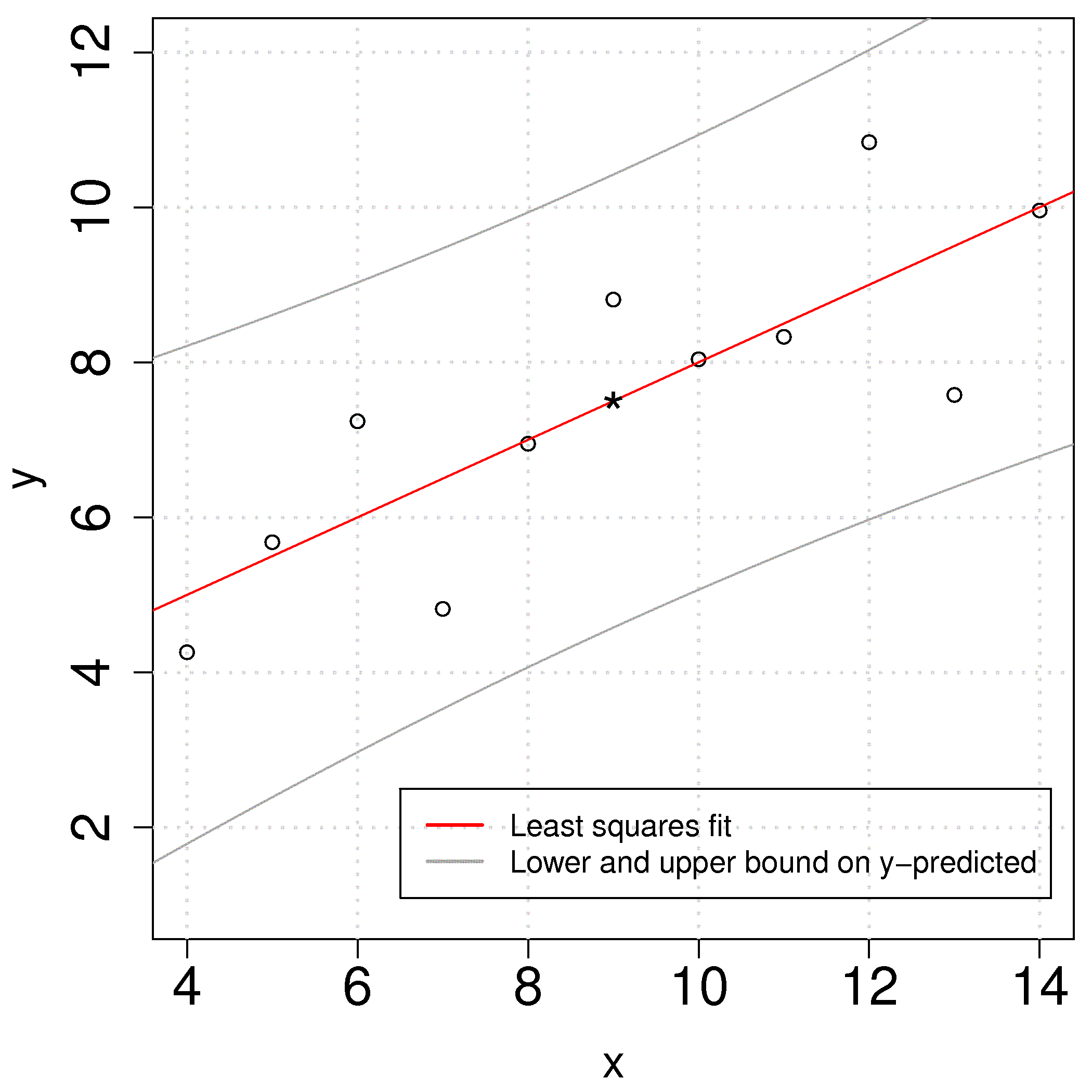
Now move left and right, away from \(\overline{\mathrm{x}}\), and mark the confidence intervals. What general shape do they have?
The prediction bounds are curved: the term \((x_i - \overline{\mathrm{x}})^2\) under the square root is smallest at the center of the model and grows as \(x_i\) moves away from \(\overline{\mathrm{x}}\) in either direction. The narrowest prediction interval therefore occurs at the center of the model, and the interval widens progressively as one moves away from the model center. This is illustrated in the figure and makes intuitive sense as well.
4.7.4. Interpretation of software output
To complete this section we show how to interpret the output from computer software packages. Most packages have very standardized output, and you should make sure that whatever package you use, that you can interpret the estimates of the parameters, their confidence intervals and get a feeling for the model’s performance.
The following output is obtained in R for the example we have been using in this section. The Python version follows below.
R, 9 lines
x <- c(10, 8, 13, 9, 11, 14, 6, 4, 12, 7, 5)
y <- c(8.04, 6.95, 7.58, 8.81, 8.33, 9.96,
      7.24, 4.26, 10.84, 4.82, 5.68)

# "Calculate for me the linear model,
# where y is described by x"
mod.ls <- lm(y ~ x)

summary(mod.ls)
and produces this output:
Output, 17 lines
Call:
lm(formula = y ~ x)

Residuals:
     Min       1Q   Median       3Q      Max
-1.92127 -0.45577 -0.04136  0.70941  1.83882

Coefficients:
            Estimate Std. Error t value Pr(>|t|)
(Intercept)   3.0001     1.1247   2.667  0.02573 *
x             0.5001     0.1179   4.241  0.00217 **
---
Signif. codes:  0 `***' 0.001 `**' 0.01 `*' 0.05 `.' 0.1 ` ' 1

Residual standard error: 1.237 on 9 degrees of freedom
Multiple R-squared: 0.6665,     Adjusted R-squared: 0.6295
F-statistic: 17.99 on 1 and 9 DF,  p-value: 0.002170
Make sure you can calculate the following values using the equations developed so far, based on the above software output:
The intercept term \(b_0\) = 3.0001.
The slope term \(b_1\) = 0.5001.
The standard error of the model, \(S_E\) = 1.237, using \(n-k = 11 - 2 = 9\) degrees of freedom.
Using the standard error, calculate the standard error for the intercept = \(S_E(b_0) = 1.1247\).
Using the standard error, calculate the standard error for the slope = \(S_E(b_1) = 0.1179\).
The \(z\)-value for the \(b_0\) term is 2.667 (R calls this the
t valuein the printout, but in our notes we have called this \(z = \dfrac{b_0 - \beta_0}{S_E(b_0)}\); the value that we compare to the \(t\)-statistic and used to create the confidence interval).The \(z\)-value for the \(b_1\) term is 4.241 (see the above comment again).
The two probability values,
Pr(>|t|), for \(b_0\) and \(b_1\) should be familiar to you; each is the probability of observing a \(z\)-value (calledt valuein the output above) at least as far from zero as the one calculated, if the true coefficient were zero. A small number is evidence the coefficient differs from zero; equivalently, the confidence interval for that coefficient does not contain zero.You can construct the confidence interval for \(b_0\) or \(b_1\) by using their reported standard errors and multiplying by the corresponding \(t\)-value. For example, if you want 99% confidence limits, then look up the 99% values for the \(t\)-distribution using \(n-k\) degrees of freedom, in this case it would be
qt((1-0.99)/2, df=9), which is \(\pm 3.25\). So the 99% confidence limits for the slope coefficient would be \([0.5 - 3.25 \times 0.1179; 0.5 + 3.25 \times 0.1179] = [0.12; 0.88]\).The \(R^2 = 0.6665\) value.
The line
F-statistic: 17.99 on 1 and 9 DFis the ratio of mean squares from the ANOVA table: \(F_0 = \dfrac{\text{RegSS}/(k-1)}{\text{RSS}/(n-k)}\) on \(k-1 = 1\) and \(n-k = 9\) degrees of freedom, with its p-value alongside.Be able to calculate the residuals: \(e_i = y_i - \hat{y}_i = y_i - b_0 - b_1 x_i\). We expect the median of the residuals to be around 0, and the rest of the summary of the residuals gives a feeling for how far the residuals range about zero.
Using Python, you can run the following code:
Python, 16 lines
import numpy as np
import statsmodels.api as sm

X = np.array([10, 8, 13, 9, 11, 14,
              6, 4, 12, 7, 5])
y = np.array([8.04, 6.95, 7.58, 8.81,
              8.33, 9.96, 7.24, 4.26,
              10.84, 4.82, 5.68])

# We do want to estimate a 'b0' term
X = sm.add_constant(X)
model = sm.OLS(y, X)
results = model.fit()
print(results.summary())
print('Standard error = {}'.format(\
    np.sqrt(results.scale)))
which produces the following output:
Output, 25 lines
                            OLS Regression Results
==============================================================================
Dep. Variable:                      y   R-squared:                       0.667
Model:                            OLS   Adj. R-squared:                  0.629
Method:                 Least Squares   F-statistic:                     17.99
Date:                Tue, 01 Jan 2019   Prob (F-statistic):            0.00217
Time:                        00:00:00   Log-Likelihood:                -16.841
No. Observations:                  11   AIC:                             37.68
Df Residuals:                       9   BIC:                             38.48
Df Model:                           1
Covariance Type:            nonrobust
==============================================================================
                 coef    std err          t      P>|t|      [0.025      0.975]
------------------------------------------------------------------------------
const          3.0001      1.125      2.667      0.026       0.456       5.544
x1             0.5001      0.118      4.241      0.002       0.233       0.767
==============================================================================
Omnibus:                        0.082   Durbin-Watson:                   3.212
Prob(Omnibus):                  0.960   Jarque-Bera (JB):                0.289
Skew:                          -0.122   Prob(JB):                        0.865
Kurtosis:                       2.244   Cond. No.                         29.1
==============================================================================


Standard error = 1.2366033227263207
As for the R code, we can see at a glance:
The intercept term \(b_0\) = 3.0001.
The slope term \(b_1\) = 0.5001.
The standard error of the model, \(S_E\) = 1.237, using \(n-k = 11 - 2 = 9\) degrees of freedom. The summary output table does not show the standard error, but you can get it from
np.sqrt(results.scale), whereresultsis the Python object from fitting the linear model.Using the standard error, calculate the standard error for the intercept = \(S_E(b_0) = 1.1247\), which is reported directly in the table.
Using the standard error, calculate the standard error for the slope = \(S_E(b_1) = 0.1179\), which is reported directly in the table.
The \(z\)-value for the \(b_0\) term is 2.667 (Python calls this the
t-value in the printout, but in our notes we have called this \(z = \dfrac{b_0 - \beta_0}{S_E(b_0)}\); the value that we compare to the \(t\)-statistic and used to create the confidence interval).The \(z\)-value for the \(b_1\) term is 4.241 (see the above comment again).
The two probability values,
P>|t|, for \(b_0\) and \(b_1\) should be familiar to you; each is the probability of observing a \(z\)-value (calledtin the output above) at least as far from zero as the one calculated, if the true coefficient were zero. A small number is evidence the coefficient differs from zero; equivalently, the confidence interval for that coefficient does not contain zero.You can construct the confidence interval for \(b_0\) or \(b_1\) by using their reported standard errors and multiplying by the corresponding \(t\)-value. For example, if you want 99% confidence limits, then look up the 99% values for the \(t\)-distribution using \(n-k\) degrees of freedom, in this case it would be
from scipy.stats import t; t.ppf(1-(1-0.99)/2, df=9), which is \(\pm 3.25\). So the 99% confidence limits for the slope coefficient would be \([0.5 - 3.25 \times 0.1179; 0.5 + 3.25 \times 0.1179] = [0.117; 0.883]\). However, the table output gives you the 95% confidence interval. Under the column0.025and0.975(leaving 2.5% in the lower and upper tail respectively). For the slope coefficient, for example, this interval is [0.233; 0.767]. If you desire, for example, the 99% confidence interval, you can adjust the code:print(results.summary(alpha=1-0.99))The \(R^2 = 0.6665\) value.
Be able to calculate the residuals: \(e_i = y_i - \hat{y}_i = y_i - b_0 - b_1 x_i\).
4.7.4.1. Visualizing the fit
Returning to the larger distillation example from the
prior section, the seaborn library has a useful function,
regplot, that draws the scatter plot of the raw data, overlays the least squares line, and
shades the confidence interval for the regression line in a single call. Note which band this is:
it is the interval for the average predicted \(\mathrm{y}\) at each \(\mathrm{x}\), and it is narrower than the
prediction interval for a single new observation, which carries the
extra \(S_E^2\) term. Software packages differ in which of the two they shade by default, so it
is worth checking.
Python, 13 lines
import pandas as pd
import seaborn as sns

distill = pd.read_csv(
    "https://openmv.net/file/distillation-tower.csv"
)

ax = sns.regplot(
    x="InvTemp3",
    y="VapourPressure",
    data=distill,
)
ax.grid(True)
A common upgrade is the jointplot, which adds a histogram (or kernel density estimate) of each
variable to the margins of the plot:
Python, 15 lines
# Marginal histograms with the regression line:
sns.jointplot(
    x="InvTemp3",
    y="VapourPressure",
    data=distill,
    kind="reg",
)

# Or the kernel density estimate:
sns.jointplot(
    x="InvTemp3",
    y="VapourPressure",
    data=distill,
    kind="kde",
)
4.7.4.2. Residuals, standard error and \(R^2\) for the model
Once the OLS model object has been fitted, the residuals on the building
data are obtained by subtracting the predictions from the observed values. Two simple summaries
of the residuals are useful: their average absolute size, and their standard deviation. Both are
“smaller is better”, and the standard deviation is the model’s standard error \(S_E\).
We continue with the model fitted in the prior section:
Python, 35 lines
# Predictions and residuals on the building data:
X_build = build[["InvTemp3"]]
y_build = build["VapourPressure"].values

prediction_build = mymodel.predict(X_build)
errors_build = y_build - prediction_build

# Average absolute residual:
avg_absolute_error = (
    pd.Series(errors_build).abs().mean()
)

# Standard deviation of the residuals
# (equivalent to S_E, up to the n-k correction):
std_error = errors_build.std()

# The standard error with the n-k degrees of
# freedom is also available directly; 2.94 kPa,
# against a spread of 6.25 kPa in the y-data:
mymodel.se_
y_build.std(ddof=1)

print(
    f"Average absolute error = "
    f"{avg_absolute_error:.3f}, "
    f"std. dev. of residuals = "
    f"{std_error:.3f}"
)

# Plot residuals in time order to look for
# trends or autocorrelation:
pd.Series(errors_build).plot(
    grid=True,
    title="Building-data residuals (Actual - Predicted)",
)
The \(R^2\) value can be read off directly from the model object, using its .score(...)
method:
Python, 2 lines
# R-squared on the building data: 0.781
mymodel.score(X_build, y_build)
As set out in the subsection on matching the metric to the purpose, a high \(R^2\) value is not a measure of prediction accuracy: it reports how strongly \(x\) and \(y\) are linearly associated. Here the model returns \(R^2 = 0.781\) on the building data, with \(S_E = 2.94\) kPa against a spread of \(s_y = 6.25\) kPa in the vapour pressure column. The prediction quality on new data is a more demanding test, and that is what we turn to in the next section.