
 Download PDF of entire book
2.15. Statistical tables for the normal- and t-distribution
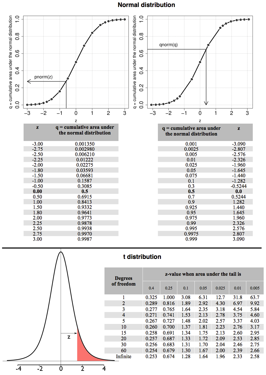
If interested, here is the code used to generate these figures
R, 92 lines
# The source code used to generate the
# *normal distribution* section:
q <- c(seq(-3.0, -2.0, 0.25),
       c(-1.8, -1.5, -1.0, -0.5, 0, 0.5,
         1.0, 1.5, 1.8),
       seq(2.0, 3.0, 0.25))
cumulative.quantile = pnorm(q)

p <- c(0.001, 0.0025, 0.005, 0.010, 0.025,
       0.05, 0.075, 0.10, 0.3, 0.5, 0.7,
       0.9, 0.925, 0.950, 0.975, 0.99,
       0.995, 0.9975, 0.999)
cumulative.probability = qnorm(p)

layout(matrix(c(1,2), 1, 2))
par(mar = c(4.2, 4.2, 0.2, 1))
plot(q, cumulative.quantile,
     type = "b",
         main = "",
         xlab = "z",
         ylab = "q = cumulative area under the normal distribution",
         cex.lab = 1.4,
         cex.main = 1.8,
         lwd = 4,
         cex.sub = 1.8,
         cex.axis = 1.8,
         ylim = c(0, 1))
grid(col="gray30")
a1 = -0.6
arrows(a1, y = -0.2, x1 = a1,
       y1 = pnorm(a1),
       code = 0, lwd = 2)
arrows(a1, y = pnorm(a1), x1 = -3,
       y1 = pnorm(a1), code = 2, lwd = 2)
text(-2, pnorm(a1) + 0.05, "pnorm(z)",
     cex = 1.5)

plot(cumulative.probability, p,
     type = "b",
         main = "",
         xlab = "z",
         ylab = "q = cumulative area under the normal distribution",
         cex.lab = 1.4,
         cex.main = 1.8,
         lwd = 4,
         cex.sub = 1.8,
         cex.axis = 1.8,
         ylim = c(0, 1))
grid(col = "gray30")
a1 = qnorm(0.65)
arrows(a1, y = 0, x1 = a1,
       y1 = pnorm(a1), code = 1, lwd = 2)
arrows(a1, y=pnorm(a1), x1 = -5,
       y1 = pnorm(a1), code = 0, lwd = 2)
text(-2, pnorm(a1)+0.05, "qnorm(q)",
    cex = 1.5)


# The source code used to generate the t-distribution section:
dof <- c(1, 2, 3, 4, 5, 10, 15, 20,
         30, 60, Inf)
tail.area.oneside <- c(0.4, 0.25, 0.1,
             0.05, 0.025, 0.01, 0.005)

n.dof <- length(dof)
n.tails <- length(tail.area.oneside)

values <- matrix(0, nrow=n.dof, ncol=n.tails)
k = 0
for (entry in tail.area.oneside){
    k = k + 1
    values[ , k] <- abs(qt(entry, dof))
}
round(values,3)

par(mar=c(4.2, 4.2, 0.2, 1))
z <- seq(-5, 5, 0.01)
probabilty <- dt(z, df=5)
plot(z, probabilty,
     type = "l",
     main = "",
     xlab = "z",
     ylab = "Probabilities from the t-distribution",
     cex.lab = 1.4,
     cex.main = 1.8,
     lwd = 4,
     cex.sub = 1.8,
     cex.axis = 1.8)
abline(h = 0)
z = 1.5
abline(v = z)
abline(v = 0)