
 Download PDF of entire book
7.11. Product development and product improvement
Most “product development” is really product improvement: new products are seldom developed from scratch. The usage examples below show what this looks like in practice, and they motivate the rest of the chapter.
7.11.1. Usage examples
Colleague: Our most high profile customer wants us to develop a product with similar, but different specifications to the prior products we have made. Is it feasible to say ‘yes’ to them?
You: we have an existing product, but a customer just wants to change one of the 7 specifications: they want a slightly higher viscosity. Keep the ingredients and ratios the same, but which process setting(s) do we change?
Manager: Keep the specifications the same, but adjust the process to use less energy and reduce emissions, even if we use slightly more expensive materials, with different ratios. Is this possible?
Engineer: A constraint has changed (e.g. a new government regulation, we have to use a different piece of equipment): how can we still get the same final product by adjusting the process conditions, or materials used in the process?
Financial controller: We can buy the raw ingredient from 4 different suppliers. Which suppliers do we pick to most cost-effectively make the product, but still achieve the specifications?
Engineer 2: Our current top line product is made with 6 different ingredients. Can we reduce this number down by adjusting the ratios or the choices of ingredients?
As these examples show, the common case is not a request for entirely new specifications, but a change to one of three things while the specifications stay the same:
which ingredients (raw materials) we use,
the ratios in which we combine them, by mass fraction, and
the process conditions used to make the product.
The methods in this chapter handle both situations — a wholly new product and the adaptation of an existing one — because the underlying problem is the same: pick values for those three groups of variables that produce the desired outcomes, using whatever historical data we have to guide the choice.
7.11.2. The three degrees of freedom
The usage examples above already named the three things we can change. Each Design step in a product-development cycle is a choice over these three groups, and the rest of the chapter keeps coming back to them, so it is worth pinning the vocabulary down explicitly.
Select the ingredients. This is a discrete choice: either an ingredient is in the recipe, or it is not. The candidate set is usually a catalogue or database of materials. In many of the usage examples above this degree of freedom is actually fixed — regulatory constraints, validation cost, or the risk of unexpected side-reactions mean we have to keep using what we already use.
Adjust the ratios of the ingredients. This is a continuous choice constrained to a simplex: the mass fractions sum to 1, so reducing one ingredient forces another to increase. This sum-to-one structure is exactly what mixture designs are built to handle.
Choose the process conditions. Temperature, pH, residence time, addition order, and the on/off state of optional steps. This is usually where the most degrees of freedom live, and where the historical data has the most correlation: temperature and flow rate, for example, are rarely independent in the historical record even when they are independent on paper.
7.11.3. Specifying the desired outcome
The desired outcome is the end goal: a vector of one or more specifications. A simple case is three scalars — a viscosity, a melting point, a density — that jointly define what “good” means.
Some entries are inequalities rather than targets: an elongation of 15 or lower is acceptable, a shelf-life of 30 days or greater is acceptable. These are yes/no constraints, and they introduce a discontinuity into the objective. Discontinuities are awkward for the optimizers later in the chapter, so we replace each one with a smoothed indicator — a sigmoid or a Gompertz function — that approximates the cliff but stays differentiable.
The desired outcome is sometimes a very long vector: a release-rate curve, a pH trajectory, an NIR spectrum. The entries in such a vector are heavily correlated, so we do not work with them directly. The first step is a principal component model of the output space; the few scores that explain it become the specification, and the rest of the methodology proceeds unchanged.
7.11.4. Product design uses every chapter of this book
The introduction to latent variable methods listed the five main areas where engineers extract value from process data:
Improved process understanding — confirming what we know, and seeing the unexpected, often by inspecting score and loading plots.
Troubleshooting process problems — isolating which variables drove a deviation, using the multivariate troubleshooting tools.
Improving, optimizing and controlling processes — moving the operating point on purpose, using designed experiments and response surface methods.
Predictive modelling — estimating a hard-to-measure quantity from the easy-to-measure ones, either with least-squares models or with inferential sensors built on PLS.
Process monitoring — raising an alarm when the process drifts away from where it should be, with univariate charts or multivariate ones.
Product design and improvement is not a sixth area. It is what happens when we do all five at once, on the same data set, in the same iteration. Each Design-Build-Test-Learn cycle (introduced below) draws on every one of them:
We start each campaign with a round of process understanding on the historical \((\mathbf{F}, \mathbf{Z}, \mathbf{Y})\) data: which materials, ratios and conditions drove the past quality outcomes? The score and loading plots of a PCA or PLS model on these matrices answer that question directly.
Each new experiment that misses the target is an act of troubleshooting: the same multivariate contribution plots that diagnose a process upset tell us which input is responsible for a missed quality target.
The improvement and optimization step is what proposes the next recipe and conditions to try. Sometimes this is a response-surface optimization on top of a designed experiment; sometimes it is mixture-design reasoning on the ratios; often it is the inverse of a PLS model, with constraints from the operating window.
Predictive models are how slow or expensive measurements — a taste panel, a 30-day shelf-life test, a customer trial — are estimated from quick lab data so the cycle does not stall waiting for the slowest test.
Monitoring in the latent-variable space tells us whether a proposed recipe is still inside the region where the historical model can be trusted, or whether the optimizer has pushed us into an extrapolated region where the predictions are not reliable.
The chapter therefore does not introduce many new techniques: it shows how to assemble the methods you already know into a single workflow that designs and improves products.
7.11.5. Why product development is difficult
Most product development is still done by intuition and trial-and-error. The methods later in this chapter can speed that work up considerably, but only if they address the things that make the problem difficult in the first place. The challenges below appear in almost every campaign, and a tool that ignores them will not improve on a good engineer’s intuition.
We frame each iteration as a Design-Build-Test-Learn (DBTL) cycle, a framing widely used in the biotechnology and autonomous-experimentation literature:
Design: pick the values for the three groups of degrees of freedom (ingredients, ratios, conditions).
Build: run one or more experiments with that design.
Test: measure the outcomes on the resulting product.
Learn: compare the outcomes against the targets, update the model, decide on the next iteration.
We do not get the product right on the first cycle, so we iterate. Even when you work by eye from plots you are running an implicit model of the system; the methods in this chapter make that model explicit, so it can be reused, criticized and improved. Six broad areas of difficulty recur — one for each stage of the cycle, plus a cross-cutting set that affects the iteration as a whole.
7.11.5.1. Problems with the specifications
The targets are usually correlated. As one increases, so does another. A specification that treats them as independent (or constrains one and lets the other float) ignores this structure and will mislead the optimization.
Specifications are often asymmetric. A weight of “ideally above 4 g” is a soft target, while “must not exceed 7 g” is a hard limit. Casting both into a single objective requires care, often using a smoothed indicator such as a sigmoid or Gompertz function.
Each DBTL cycle is solved as an optimization, so we have to capture several targets in a single objective. Sum of squared deviations? Absolute deviations? Equal weights, or a ranking? And how do we scale a target measured in 1000s so it does not swamp one measured in 0.01s?
Profit is often suggested as the objective, but reliable estimates of selling price, raw-material costs, emissions, labour and rework costs are rarely all available at the same time.
Closeness to a lab-scale specification is not the same as robustness in production or in the customer’s hands. An optimum found in the lab can perform poorly at full scale.
7.11.5.2. Problems in the Design step
The first iteration has little or no data, so the search direction has to come from prior knowledge or screening designs.
When experiments can run in parallel (e.g. on a robotic platform), how many points, where in the input space, and with how many replicates?
Step size matters. Moving from \(x = 0.5\) to \(x = 0.499\) is wasteful; moving to \(x = 0.2\) may be too far. The right step balances information against cost, and we would like that choice to be automatic in a self-driving DBTL loop.
Bringing in new candidate ingredients is a combinatorial problem. With 100 candidate plastics it helps to rank them on a continuous scale (e.g. thermal stability) so the choice becomes a numeric variable rather than a 100-way switch.
On/off effects: the mere presence of an ingredient at small amounts can flip the system’s behaviour, creating strong nonlinearities that are hard to model.
Process conditions are sometimes discrete (stirrer at off / low / high), and the order of manufacturing steps matters.
Model inversion is non-unique. Solving \(x + y = 4\) has infinitely many solutions, and product design almost always has more inputs (manipulated variables) than outputs (targets), so the inverse problem is underdetermined.
7.11.5.3. Problems in the Build step
How repeatable can you run the same recipe? Without good control here an apparent improvement may just be experimental noise, and a move to a new operating region cannot be distinguished from drift.
Even when a recipe is reproduced perfectly, there are block effects between iterations. Including references and controls in each cycle lets us correct for these.
Is the lab system a faithful proxy for how the customer actually uses the product? A product that is robust on the bench and fails in customer hands has not really been improved.
7.11.5.4. Problems in the Test step
Measurement reproducibility. Outputs sometimes shift between iterations because of uncontrolled factors. We would like to eliminate those factors, or at least correct for them.
Outputs interact. Viscosity readings depend on pH, for example, so the test result is itself a function of more than one quality.
Sensory and slow lab measurements cannot be done on every experiment. A taste panel, or a 5-day shelf-life test, will not keep up with a fast iteration loop. Inferential sensors and other surrogate measurements speed up the cycle, but they introduce their own error.
7.11.5.5. Problems in the Learn step
Which way do we go next: explore an unexamined region, or exploit the neighbourhood of the current best result? And how should the balance shift as we accumulate cycles?
Which model family should we use for the forward (inputs to outputs) prediction: Gaussian processes, polynomial response surfaces, splines, latent variable models? Which can be inverted analytically, and which require an optimization to invert?
When do we drop old data; when is a surprising point an outlier and not the next ah-ha result; and how do we use the model’s predictive uncertainty to decide where to sample next?
7.11.5.6. Problems with the cycle itself
When do we stop? The obvious case is when the goal is reached, but we also need to detect diminishing returns, and to recognize when no feasible solution exists.
An optimum sits in a nonlinear region by definition. How do we know we have found the global peak rather than a local one?
Storage and provenance. How do we name experiments, record ratios and units, and capture covariates (ambient humidity, operator, lot numbers, raw-material amounts that were “constant”) that we did not think mattered until the day they did? Model versioning, input-data lineage and a clear audit trail are part of this discipline.
7.11.5.7. What we ask of an ideal framework
The difficulties above tell us what an ideal framework needs to do. Most of those properties — handling correlated and high-dimensional outputs, tolerating missing data, working from small experimental sets, balancing exploration against exploitation, supporting model inversion — are addressed directly by the methods later in this chapter and the cross-references above. Four further properties cut across the whole cycle and are worth stating explicitly:
Guided by the subject matter expert. The tool accelerates the expert; it does not replace them. The SME specifies constraints, vetoes infeasible suggestions, and chooses between alternative solutions when the inversion is non-unique.
Inductive, not transductive. The model must generalize to new ingredients, conditions and properties — not just interpolate within the training set. This is why we represent the recipe through a property database (the \(\mathbf{D}\) matrix in the next section), rather than as a categorical choice between named materials. See the transduction entry for the contrast with the inductive case.
Interpretable. The results must be understandable to the expert: they should confirm prior knowledge where it exists, and surface new insight where it does not. Score and loading plots from PCA and PLS are the workhorses here, which is one reason we lean on latent variable methods for the rest of the chapter.
Reports an operating window. When constraints are active at a solution, the framework names them, so we learn the limits of the system. When constraints are inactive, the directions in which we can move without losing the solution are reported as an operating window, and ideally the solution is parameterised so the SME can fine-tune within that window. Multivariate troubleshooting tools give us the same diagnostic in the latent-variable space.
The remainder of this chapter shows how the methods already developed in the book — designed experiments, response surface methods and latent variable models, together with standard and Bayesian optimization — deliver against these properties.
Three further goals are sometimes asked of a product-development framework but are not treated rigorously here: handling large data sets, transfer learning across manufacturing sites, and a formal proof of permutation invariance. The methods we use cope with each of them informally — latent-variable models scale to large \(N\), mean-centring and scaling are insensitive to row order in practice, and a model trained on one site can be re-fit at another — but a careful treatment is left to the literature.
7.11.6. Data needed for product development
The methods later in this chapter operate on four data tables that fit together. We refer to them by capital letters: \(\mathbf{D}\), \(\mathbf{F}\), \(\mathbf{Z}\) and \(\mathbf{Y}\). Each table answers a different question and each one normally comes from a different source. Setting them up correctly — and getting the alignment between them right — is most of what makes the rest of the workflow possible.
\(\mathbf{D}\): a property database, one column per candidate building block, one row per measured property.
\(\mathbf{F}\): a recipe table, one row per experiment, columns aligned with \(\mathbf{D}\), entries are mass fractions that sum to 1.
\(\mathbf{Z}\): a process-conditions table, one row per experiment, columns are the conditions used to make that row’s product.
\(\mathbf{Y}\): a quality-outcomes table, one row per experiment, columns are the KPIs that the customer (or our specification) cares about.
The matrix \(\mathbf{D}\) shares columns with \(\mathbf{F}\). The matrices \(\mathbf{F}\), \(\mathbf{Z}\) and \(\mathbf{Y}\) share rows: row \(i\) of each describes the same experiment.
7.11.6.1. The property database \(\mathbf{D}\)
This is the most heterogeneous of the four. Each column of \(\mathbf{D}\) is a candidate building block — an oil, a fat, a binder, a filler, a polymer — and the rows are properties: molecular weight, melting point, viscosity at a given shear rate, surface tension, NIR absorbance at each wavelength, and so on. Some practitioners prefer the transposed layout (one material per row, properties as columns); either is fine, as long as you stay consistent.
\(\mathbf{D}\) is assembled from internal lab measurements, supplier data sheets, public databases, and computational property estimators. It is worth investing in: a well-populated \(\mathbf{D}\) is reused across many product-development campaigns. Collect more rows and more columns than you strictly need for the current project.
A few practical points:
Do not break “compound” ingredients into their pure constituents. If you use milk as an ingredient, store the properties of milk; do not try to split it into water, fat, protein and lactose. The same goes for any pre-mix or proprietary blend. The columns of \(\mathbf{D}\) should match the units in which you actually purchase, weigh and add the materials — the same units that appear in \(\mathbf{F}\).
Properties are usually blocked. Some rows are only meaningful for solids, others only for liquids, others only for spectroscopic samples. The methods in this chapter handle missing values explicitly, as long as you mark them as missing rather than filling with zeros.
The result must not depend on the order of rows or columns. We may group rows — for example, all NIR wavelengths together — so that block-wise preprocessing is possible, but inside a group the order is arbitrary. This is one of the desiderata (item M) in the previous section.
Vector-valued properties belong in :math:`mathbf{D}` as consecutive rows: a particle-size distribution, a thermogravimetric trace, an NIR spectrum. Such blocks are highly correlated and are a natural fit for a principal component model.
7.11.6.2. The recipe \(\mathbf{F}\)
Each row of \(\mathbf{F}\) is one experiment or one product, and each column is a building block, aligned with the columns of \(\mathbf{D}\). The entries in a row are mass fractions and typically sum to 1.
The rows in \(\mathbf{F}\) need not be products that you sell. Intermediate blends, side experiments and customer trials all belong, as long as each row has a corresponding outcome in \(\mathbf{Y}\). It is also useful to split \(\mathbf{F}\) into sub-blocks — a binders block, a fats block, a starches block — so that the model can later assess the effect of each material family separately.
7.11.6.3. The process conditions \(\mathbf{Z}\)
The matrix \(\mathbf{Z}\) has the same number of rows as \(\mathbf{F}\) and one column per process condition: temperature, pressure, mixing speed, residence time, addition order. Discrete settings (a stirrer that is off, low or high) are one-hot encoded. Recipe steps that may or may not be applied are stored as 0/1 indicators.
It is tempting to leave \(\mathbf{Z}\) out when only the recipe varies during a campaign. Resist that temptation. Conditions that look constant in a campaign — ambient humidity, operator, raw-material lot number, the calibration date of the analyser — routinely turn out, after the fact, to have driven a result. If they were never recorded, that diagnosis is impossible. (When such effects are expected and we want to remove them by design, we can plan the campaign with blocking.) The correct rule is: store the suspected covariates as well as the obvious controlled variables, even if you do not plan to vary them.
7.11.6.4. The quality outcomes \(\mathbf{Y}\)
Each row of \(\mathbf{Y}\) is the same experiment as the corresponding row of \(\mathbf{F}\) and \(\mathbf{Z}\). The columns are the key performance indicators (KPIs): viscosity, melting point, shelf life, taste-panel score, and so on. Vector outcomes (such as a release-rate curve) can also be stored in \(\mathbf{Y}\) as consecutive columns; if they are highly correlated, summarize them with a few principal components first.
The crucial design rule for \(\mathbf{Y}\) is to capture, at minimum, the same metrics the customer specifies. The whole point of the methodology is to invert the relationship \((\mathbf{D}, \mathbf{F}, \mathbf{Z}) \rightarrow \mathbf{Y}\) so that, given a target row \(\mathbf{y}_\text{new}\), we can prescribe the recipe and conditions \((\mathbf{f}_\text{new}, \mathbf{z}_\text{new})\) that achieve it. If the customer’s target metrics are not among the columns of \(\mathbf{Y}\), the inversion is solving the wrong problem.
As with \(\mathbf{D}\), capture provenance for every entry: who measured the value, where, when, in which units, and with which protocol. Two viscosity numbers measured with different geometries are not the same measurement.
7.11.6.5. How the four tables fit together
\(\mathbf{D}\) and \(\mathbf{F}\) share columns. Every ingredient appearing in any recipe must have a property column in \(\mathbf{D}\). A new, unseen ingredient can later be added to \(\mathbf{D}\) and then used in \(\mathbf{F}\), provided its properties lie within the correlation structure of the existing materials.
\(\mathbf{F}\), \(\mathbf{Z}\) and \(\mathbf{Y}\) share rows. Row \(i\) of each describes the same experiment, so they can be concatenated horizontally for a multi-block PLS analysis. Standard preprocessing (mean-centring, scaling, optional block scaling) applies before the model is built.
The forward model \((\mathbf{F}, \mathbf{Z}) \rightarrow \mathbf{Y}\) is augmented by the property information in \(\mathbf{D}\), so that the model is expressed in terms of what the materials do (their physical and chemical properties), not just which materials were chosen. This is what allows the model to generalize to new ingredients — the inductive property (item D) of the desiderata.
Inversion of this model is generally underdetermined: there are typically more inputs than outputs, so a target \(\mathbf{y}_\text{new}\) corresponds to a region of feasible \((\mathbf{f}_\text{new}, \mathbf{z}_\text{new})\) rather than a single point. The dimension of that region is the difference between the rank of the input space and the rank of the output space (the “rank” idea in the previous subsection); the inactive directions are the operating window described by item J of the desiderata.
7.11.7. Optimizing: new operating point and/or new product development
This application area is rapidly growing in importance. Fortunately it is fairly straightforward to get an impression of how powerful this tool is. Let’s return back to the food texture example considered previously, where data from a biscuit/pastry product was considered. These 5 measurements were used:
Percentage oil in the pastry
The product’s density (the higher the number, the more dense the product)
A crispiness measurement, on a scale from 7 to 15, with 15 being more crispy.
The product’s fracturability: the angle, in degrees, through which the pasty can be slowly bent before it fractures.
Hardness: a sharp point is used to measure the amount of force required before breakage occurs.
The scores and loadings plot are repeated here again:
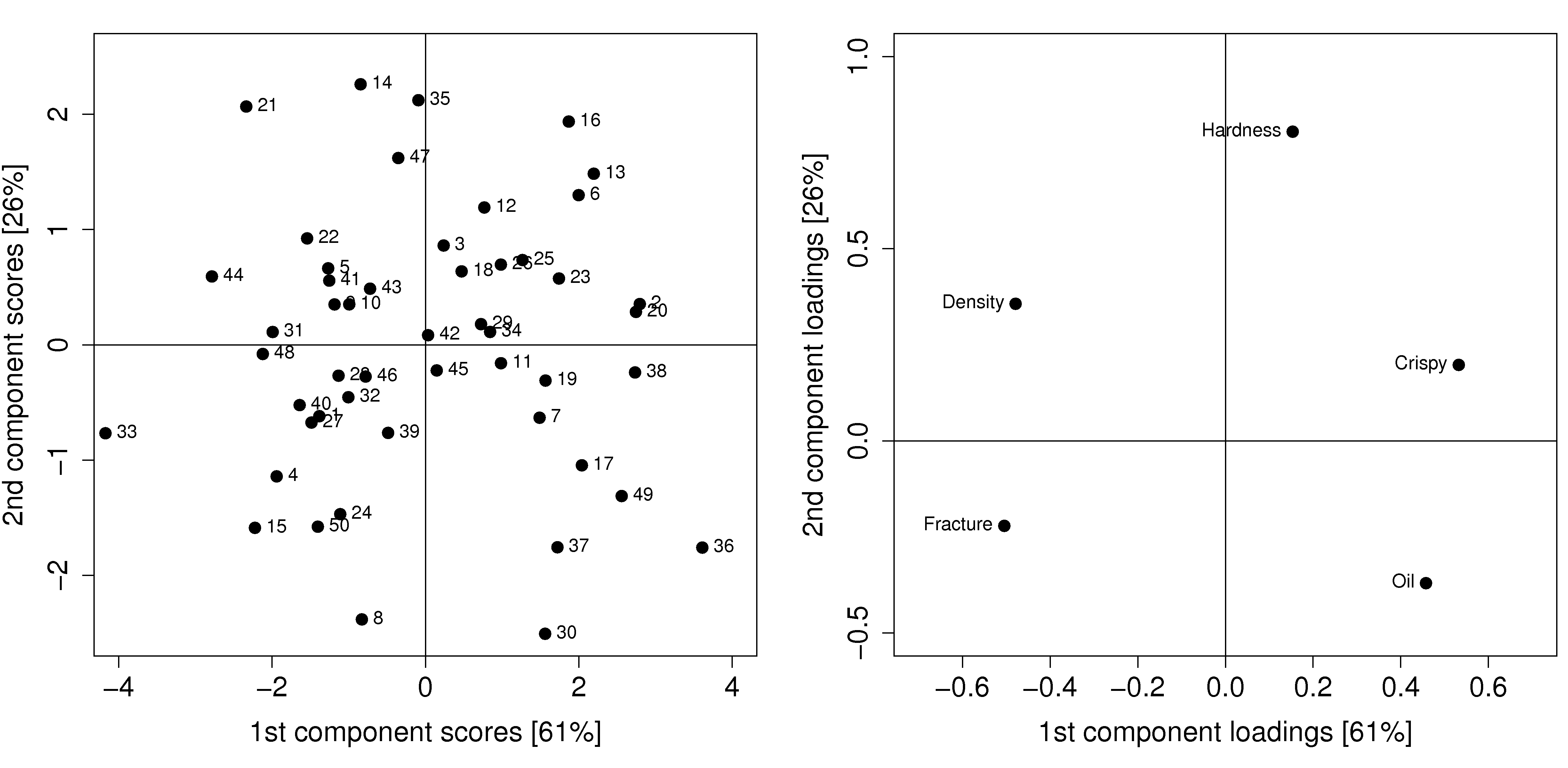
Process optimization follows the principle that certain regions of operation are more desirable than others. For example, if all the pastry batches produced on the score plot are of acceptable quality, there might be regions in the plot which are more economically profitable than others.
For example, pastries produced in the lower right quadrant of the score plot (high values of \(t_1\) and low values of \(t_2\)), require more oil, but might require a lower cooking time, due to the decreased product density. Economically, the additional oil cost is offset by the lower energy costs. All other things being equal, we can optimize the process by moving production conditions so that we consistently produce pastries in this region of the score plot. We could cross-reference the machine settings for the days when batches 17, 49, 36, 37 and 30 were produced and ensure we always operate at those conditions.
New product development follows a similar line of thought, but uses more of a “what-if” scenario. If market research or customer requests show that a pastry product with lower oil, but still with high crispiness is required, we can initially guess from the loadings plot that this is not possible: oil percentage and crispiness are positively correlated, not negatively correlated.
But if our manager asks, can we readily produce a pastry with the 5 variables set at [Oil=14%, Density=2600, Crispy=14, Fracture can be any value, Hardness=100]. We can treat this as a new observation, and following the steps described in the earlier section on using a PCA model, we will find that \(\mathbf{e} = [2.50, 1.57, -1.10, -0.18, 0.67]\), whose sum of squares is 10.4; the SPE value is the square root of that sum, 3.22, which is the scale on which the process_improve package reports SPE so that it compares with the limit from spe_limit. This is well above the 95% limit of SPE, indicating that such a pastry is not consistent with how we have run our process in the past. So there isn’t a quick solution.
Fortunately, there are systematic tools to move on from this step. They involve the inversion of a latent variable model: running the model backwards, from a desired result to the recipe that would produce it. The worked example below introduces the idea on the food texture data. A good starting point for further reading is the paper by Christiane Jaeckle and John MacGregor, “Product design through multivariate statistical analysis of process data”. AIChE Journal, 44, 1105-1118, 1998.
The general principle in model inversion problems is to manipulate the any degrees of freedom in the process (variables that can be manipulated in a process control sense) to obtain a product as close as possible to the required specification, but with low SPE in the model. A PLS model built with these manipulated variables, and other process measurements in \(\mathbf{X}\), and collecting the required product specifications in \(\mathbf{Y}\) can be used for these model inversion problems.
7.11.8. Worked example: PCA model inversion
The previous section ended with a manager’s question: what recipe will give us the pastry we want? A latent variable model can be run in reverse to answer it. This is called model inversion. The forward calculation takes a new observation and projects it onto the model to obtain its scores; inversion does the opposite, starting from a desired score and recovering the raw variables that would place an observation there.
For a two-component PCA model the idea is geometric. The model is a flat plane embedded in the five-dimensional space of pastry properties, and every pastry projects onto that plane at a score \((t_1, t_2)\). To invert the model we choose a target score and read off the point on the plane it corresponds to. With the loadings matrix \(\mathbf{P}\) (here \(5 \times 2\)) and a target score \(\mathbf{t} = [t_1, t_2]\):
This result is in the model’s mean-centered and scaled units; undoing the centering and scaling returns a recipe in the original units of percentage oil, density, and so on.
We build the model on the same food texture data as before, mean-centered and scaled to unit variance:
Python, 9 lines
import numpy as np
import pandas as pd
import plotly.graph_objects as go
from plotly.subplots import make_subplots
from process_improve.multivariate import PCA, MCUVScaler

food = pd.read_csv("https://openmv.net/file/food-texture.csv", index_col=0)
scaler = MCUVScaler().fit(food)
food_mcuv = scaler.transform(food)
Two components are enough for this small data set:
Python, 3 lines
A = 2
model = PCA(n_components=A).fit(food_mcuv)
print(model.r2_cumulative_)
The first component explains 60.6% of the variability in the five measurements and the second a further 25.9%, for a cumulative \(R^2\) of 86.5%.
Before trusting the model to generate recipes, we should check that it is a faithful summary of the data. We plot the SPE and Hotelling’s \(T^2\) value of each pastry, together with their 95% limits:
Python, 21 lines
spe = model.spe_.iloc[:, -1]
t2 = model.hotellings_t2_.iloc[:, -1]
spe_limit = float(model.spe_limit(conf_level=0.95))
t2_limit = float(model.hotellings_t2_limit(conf_level=0.95))

fig = go.Figure()
fig.add_trace(go.Scatter(y=spe.values, mode="lines+markers", name="SPE"))
fig.add_hline(y=spe_limit, line_color="red", line_dash="dash",
              annotation_text="95% limit")
fig.update_layout(title="SPE per pastry", xaxis_title="Pastry number",
                  yaxis_title="SPE", height=320)
fig.show()

fig = go.Figure()
fig.add_trace(go.Scatter(y=t2.values, mode="lines+markers", name="T2"))
fig.add_hline(y=t2_limit, line_color="red", line_dash="dash",
              annotation_text="95% limit")
fig.update_layout(title="Hotelling's T-squared per pastry",
                  xaxis_title="Pastry number", yaxis_title="T-squared",
                  height=320)
fig.show()


The 95% limits work out to \(\text{SPE} = 1.38\) and \(T^2\) \(= 6.65\). Two pastries sit just above the SPE limit and one just above the \(T^2\) limit — about what a 95% limit implies for 50 observations, and none is a gross outlier. The two-component plane is a sound summary of how this product has been made, so it is a sensible basis for inversion.
The score plot is the model’s two-dimensional map of the data, and the loadings give that map its meaning:
Python, 21 lines
scores = model.scores_
ci_x, ci_y = model.ellipse_coordinates(score_horiz=1, score_vert=2,
                                       conf_level=0.95)

fig = make_subplots(rows=1, cols=2, subplot_titles=("Scores", "Loadings"))
fig.add_trace(go.Scatter(x=scores.iloc[:, 0], y=scores.iloc[:, 1],
                         mode="markers", marker=dict(color="black"),
                         showlegend=False), row=1, col=1)
fig.add_trace(go.Scatter(x=ci_x, y=ci_y, mode="lines",
                         line=dict(color="palevioletred"),
                         showlegend=False), row=1, col=1)
fig.add_trace(go.Scatter(x=model.loadings_.iloc[:, 0],
                         y=model.loadings_.iloc[:, 1], mode="markers+text",
                         text=model.loadings_.index,
                         textposition="bottom center",
                         showlegend=False), row=1, col=2)
fig.update_xaxes(title_text="t1", row=1, col=1)
fig.update_yaxes(title_text="t2", row=1, col=1)
fig.update_xaxes(title_text="p1", row=1, col=2)
fig.update_yaxes(title_text="p2", row=1, col=2)
fig.show()

Earlier we noted that the lower-right quadrant of the score plot — high \(t_1\), low \(t_2\) — is the economically attractive region. Model inversion turns a chosen point in that quadrant into a concrete recipe. We extract the loadings as a plain array and project a target score back through them:
Python, 10 lines
P = model.loadings_.values

def invert(t1, t2):
    """Return the pastry recipe for a target score (t1, t2)."""
    x_scaled = np.array([[t1, t2]]) @ P.T
    recipe = scaler.inverse_transform(pd.DataFrame(x_scaled, columns=food.columns))
    return recipe.iloc[0]

print(invert(0, 0))     # the origin returns the average pastry
print(invert(2, -1))    # a point in the profitable quadrant
Inverting the origin \((0, 0)\) returns Oil = 17.2%, Density = 2858, Crispy = 11.5, Fracture = 20.9, Hardness = 128. These are the column means: a useful sanity check, since the centre of the score plot must correspond to the average pastry.
The target \((t_1 = 2,\ t_2 = -1)\) inverts to a recipe of Oil = 19.2%, Density = 2694, Crispy = 13.1, Fracture = 16.6, Hardness = 113. Next to the average pastry this one is oilier, less dense, and crispier — exactly the trade-off the loadings plot predicts for that quadrant, now written as numbers a process engineer can aim for.
Two cautions apply. First, a target is only realistic if it lies within the model: inside the \(T^2\) ellipse, and implying a low SPE. Asking for a score far outside the cloud of pastries inverts to a recipe the process has never been shown to produce. Second, the inversion above is unconstrained — it is free to move all five variables at once. In practice some variables are fixed (a hardness specification, say) and the rest must be solved for. We work through that case next.
A recipe is often not free in every variable. A product specification may fix one of them — suppose a customer requires the hardness to come out at an exact value. The model still has only two score degrees of freedom, \(t_1\) and \(t_2\). Pinning one variable adds one equation that those two scores must satisfy, so it uses up one degree of freedom: we are no longer free to roam the whole score plane, only a line within it.
Each scaled variable is reconstructed from the scores through its own row of the loadings matrix \(\mathbf{P}\). Writing \(\mathbf{p}_h = [p_{h,1},\ p_{h,2}]\) for the hardness row, the hardness of any point on the model plane is
where \(z_h\) is the desired hardness, expressed in the model’s mean-centered and scaled units. Fixing \(z_h\) turns this into the equation of a straight line in the \((t_1, t_2)\) plane: every score on that line reproduces the requested hardness exactly.
We still have a target score in mind — the profitable point \(\mathbf{t}^\star = (2, -1)\) from before — but in general it does not lie on the constraint line. To find the score we should use instead, split the target into two parts: the component pointing along the hardness loading direction \(\mathbf{p}_h\), and the component perpendicular to it. Only the first part changes the hardness — the perpendicular component contributes nothing to the dot product \(\mathbf{p}_h \cdot \mathbf{t}\). So we keep the perpendicular part of the target exactly as it is, and reset only the along-\(\mathbf{p}_h\) part, choosing it so the hardness comes out at the requested value. Holding the perpendicular component fixed moves the score as little as the constraint allows.
That operation — keep the perpendicular part, reset the part along \(\mathbf{p}_h\) — is the orthogonal projection of the target \(\mathbf{t}^\star\) onto the constraint line. It shifts the target along \(\mathbf{p}_h\):
The numerator is the amount by which the unconstrained target misses the required hardness; the correction \(\lambda\,\mathbf{p}_h\) is subtracted from the target scores to bring them onto the constraint line. The further the requested hardness is from what the target naturally gives, the larger \(\lambda\), and the more the other four variables must move to compensate.
Fixing one variable used up only one of the two score degrees of freedom; the second is still ours to spend. Projection spends it on staying as close to the original target as possible — the perpendicular component of the target is carried over untouched. That is the natural default, but not the only choice: we could instead hold \(t_1\) at its target value and solve \(t_2\) alone for the required hardness, which gives a different recipe that is equally, and exactly, at the requested hardness. Whenever a constraint leaves a degree of freedom unclaimed, some rule has to decide how to use it.
Python, 13 lines
p_h = model.loadings_.loc["Hardness"].values   # the hardness loadings row

def invert_fixing_hardness(t_star, hardness):
    """Invert towards t_star, but force Hardness to an exact value."""
    z_h = (hardness - scaler.center_["Hardness"]) / scaler.scale_["Hardness"]
    t_star = np.array(t_star, dtype=float)
    lam = (p_h @ t_star - z_h) / (p_h @ p_h)
    t = t_star - lam * p_h
    recipe = scaler.inverse_transform(pd.DataFrame([t @ P.T], columns=food.columns))
    return recipe.iloc[0]

print(invert_fixing_hardness([2, -1], 110))
print(invert_fixing_hardness([2, -1], 150))
The unconstrained target \((2, -1)\) already gave a hardness of 113, so asking for 110 barely disturbs anything: the correction is tiny (\(\lambda = 0.13\)) and the other four variables are essentially unchanged — Oil = 19.3%, Density = 2691, Crispy = 13.0, Fracture = 16.7, against the unconstrained 19.2, 2694, 13.1, 16.6. The model is telling us this hardness was almost free.
Asking for a hardness of 150 is a different matter. It is well above what the target naturally produces, so the correction is large (\(\lambda = -1.79\)) and the scores swing all the way from \(t_2 = -1\) to \(t_2 = +0.4\). The recipe becomes Oil = 18.6%, Density = 2741, Crispy = 13.8, Fracture = 14.1, Hardness = 150 — every other variable has moved to pay for the harder pastry. This is the model’s honest answer: there is no recipe close to the original target that is also that hard, so something has to give.
This projection geometry is easiest to see drawn. The score plane below shows the target \(\mathbf{t}^\star\), the two constraint lines, and the correction that lands the target on each — short for the nearby hardness of 110, long for the distant hardness of 150:

To explore the inversion interactively — hovering over any target in the score plot and reading off the recipe it implies — download and run this notebook: PCA-model-inversion.ipynb.
7.11.9. References
The four-table organization is drawn from a sequence of papers, several of whose authors I have had the pleasure of working with over the past 25 years:
Salvador García-Muñoz, “Two Novel Methods to Analyze the Combined Effect of Multiple Raw-Materials and Processing Conditions on the Product’s Final Attributes: JRPLS and TPLS.” Chemometrics and Intelligent Laboratory Systems, 133, 2014, https://doi.org/10.1016/j.chemolab.2014.02.006
Koji Muteki, John F. MacGregor and Toshihiro Ueda, “Mixture Designs and Models for the Simultaneous Selection of Ingredients and Their Ratios.” Chemometrics and Intelligent Laboratory Systems, 86, 2007.
Christiane M. Jaeckle and John F. MacGregor, “Product Design through Multivariate Statistical Analysis of Process Data.” AIChE Journal, 44, 1998.
Emanuele Tomba, Massimiliano Barolo and Salvador García-Muñoz, “General Framework for Latent Variable Model Inversion for the Design and Manufacturing of New Products.” Industrial & Engineering Chemistry Research, 51, 2012, https://doi.org/10.1021/ie301214c