5.20. A worked screen-then-optimise study: six factors on a reactor with a heat limit

Screening and optimising ask different questions of a process, so a study that does both can design each stage for its own question. The screen has to separate the few factors that matter from those that do not, in as few runs as possible. The optimisation has to predict well wherever the best settings might lie, and that region is not always the cube a classical design fills: a limit the process must respect can cut a corner off it.

This section runs both stages on a simulated reactor whose true behaviour is known, so the recommended settings can be scored against the best ones available. It uses 36 runs in three steps:

• a 17-run definitive screening design in six factors, analysed with the staged analysis;

• a 16-run optimal design in the three factors that matter, built inside a heat-release limit;

• three confirmation runs at the settings with the highest overall desirability.

5.20.1. The process and the question

A catalytic reaction is run in batches in a stirred, jacketed reactor. The yield of product is to be as high as possible, and the impurity must stay below 2.0%, the level at which a batch is rejected. Six factors might matter:

Factor	Low	High
Temperature \(T\), °C	150	200
Reaction time \(t\), min	10	40
Catalyst loading \(C\), mol%	0.5	2.0
Pressure \(P\), bar	2	10
Stirrer speed \(S\), rpm	300	900
Feed molar ratio \(R\)	1.0	1.5

The screening runs are made in a laboratory reactor and the optimisation runs in the pilot reactor, where one more limit applies. The heat a batch releases grows with the volume of the reacting mass, while the heat the cooling jacket removes grows with the jacket’s area, and for vessels of the same shape the area per unit of volume falls as the vessel gets larger. A recipe that the laboratory reactor cools easily can therefore release heat faster than the pilot reactor’s jacket can remove it.

The heat released rises with both temperature and catalyst loading. Over the corner of the factor ranges where it exceeds the jacket’s capacity, the plant engineers approximate the limit by a straight line,

\[0.04\,T + C \le 9.5\]

with \(T\) in °C and \(C\) in mol%. At 200 °C the catalyst loading cannot exceed 1.5 mol%, while at 187.5 °C and below every loading in the range is allowed.

5.20.2. A simulator in place of the reactor

The simulator’s true models are written out in the code below, in coded units, where each factor runs from \(-1\) at its low setting to \(+1\) at its high setting. Only temperature, reaction time and catalyst loading affect the responses; pressure, stirrer speed and feed ratio do not. Each batch adds noise with a standard deviation of 0.5 percentage points on the yield and 0.05 percentage points on the impurity. The simulator gives both reactors the same chemistry, so the heat limit is the only difference between them.

The analysis sees only the simulated measurements; the true models are used once, at the end, to score the answer. Every figure in this section is reproducible with process_improve. Each block imports what it needs and reuses variables from the blocks before it, so paste them in order.

Python, 52 lines

import numpy as np
import pandas as pd
import plotly.graph_objects as go
from patsy import dmatrix
from plotly.subplots import make_subplots

from process_improve.experiments import (
    Constraint, DesignRegion, Factor, analyze_experiment, analyze_omars, evaluate_design,
    generate_design, optimize_responses,
)

factors = [
    Factor(name="T", low=150, high=200, units="degC"),   # temperature
    Factor(name="t", low=10, high=40, units="min"),      # reaction time
    Factor(name="C", low=0.5, high=2.0, units="mol%"),   # catalyst loading
    Factor(name="P", low=2, high=10, units="bar"),       # pressure
    Factor(name="S", low=300, high=900, units="rpm"),    # stirrer speed
    Factor(name="R", low=1.0, high=1.5),                 # feed molar ratio
]
names = [f.name for f in factors]

# The ten terms of a quadratic model in T, t and C, named as analyze_experiment names them.
QUADRATIC = "T + t + C + T:t + T:C + t:C + I(T ** 2) + I(t ** 2) + I(C ** 2)"
# The simulator's true coefficients, in coded units. P, S and R appear in neither model.
TRUE_MODELS = {
    "yield": {"Intercept": 70, "T": 6, "t": 4, "C": 5, "T:C": 2.5,
              "I(T ** 2)": -3, "I(t ** 2)": -2, "I(C ** 2)": -1.5},
    "impurity": {"Intercept": 1.6, "T": 0.2, "t": 0.5, "C": 0.1, "I(t ** 2)": 0.3},
}
NOISE_SD = {"yield": 0.5, "impurity": 0.05}   # batch to batch, in percentage points

def quadratic_terms(settings):
    """The quadratic model's terms at settings in actual units, coded -1 (low) to +1 (high).

    Only the first three factors, T, t and C, enter the models.
    """
    coded = pd.DataFrame({f.name: (settings[f.name] - (f.low + f.high) / 2)
                                  / ((f.high - f.low) / 2) for f in factors[:3]})
    return dmatrix(QUADRATIC, coded, return_type="dataframe")

def true_response(settings):
    """Yield and impurity, in %, without noise."""
    X = quadratic_terms(settings)
    return pd.DataFrame({r: X[list(model)] @ pd.Series(model)
                         for r, model in TRUE_MODELS.items()})

rng = np.random.default_rng(2026)

def run_reactor(settings):
    """One batch at each row of settings: the true response plus batch-to-batch noise."""
    noise = {r: rng.normal(0, sd, len(settings)) for r, sd in NOISE_SD.items()}
    return true_response(settings) + pd.DataFrame(noise, index=settings.index)

Run in browser

5.20.3. Finding the factors that matter, in seventeen runs

A definitive screening design with fake factors tests each main effect against an error estimate that no quadratic or interaction effect can bias. The smallest definitive screening design for six factors has 13 runs, a conference matrix of order 6, its mirror image and a centre run, and leaves no column for a fake factor. Asking for 17 runs builds the design from a conference matrix of order 8 instead, and the two columns that no factor is assigned to are the fake factors. The foldover makes every main-effect column, the fake ones included, orthogonal to every quadratic and interaction column, so with no third-order effects present the fake factors pick up only noise. They give the analysis 2 degrees of freedom for error before anything is assumed about which effects are active.

Python, 8 lines

screen = generate_design(factors, "dsd", budget=17, random_state=1)
print(screen.n_runs, screen.metadata["conference_order"], screen.metadata["fake_factors"])
# 17 8 2

# Every main-effect column is orthogonal to every quadratic and interaction column.
x = screen.design[names].to_numpy(float)
second_order = np.column_stack([x[:, i] * x[:, j] for i in range(6) for j in range(i, 6)])
print(np.abs(x.T @ second_order).max())   # 0.0

Run in browser

The staged analysis tests the main effects first, against the fake-factor error estimate. It then pools the inactive main effects into that estimate and searches for second-order terms among the factors whose main effects are active. With strong heredity, a quadratic or interaction may enter only if the main effects of its factors are active. Both responses are analysed, since the second experiment has to model both.

Python, 13 lines

screen_obs = run_reactor(screen.design_actual)
for response in ["yield", "impurity"]:
    staged = analyze_omars(screen.design[names], screen_obs[response],
                           quadratic_heredity="strong", interaction_heredity="strong")
    p = ", ".join(f"{name} {value:.2g}" for name, value in staged.main_effect_p_values.items())
    terms = staged.active_main_effects + staged.active_quadratics + staged.active_interactions
    print(f"{response}: error df {staged.initial_error_df} then {staged.updated_error_df}; "
          f"p-values {p}")
    print(f"  selected: {terms}")
# yield: error df 2 then 5; p-values T 0.00031, t 0.00067, C 0.00048, P 0.68, S 0.9, R 0.97
#   selected: ['T', 't', 'C', 'T^2', 't^2', 'C^2', 'T:C']
# impurity: error df 2 then 5; p-values T 0.00088, t 0.0001, C 0.0023, P 0.11, S 0.27, R 0.9
#   selected: ['T', 't', 'C', 't^2']

Run in browser

Both responses separate the factors the same way. Temperature, reaction time and catalyst loading have p-values below 0.003, and pressure, stirrer speed and feed ratio have p-values of 0.11 or more. The second-order terms selected are exactly those in the simulator’s models, a check that only a simulation allows.

For the team, the second experiment needs three factors instead of six, and pressure, stirrer speed and feed ratio can be held wherever is most convenient.

That experiment fits the full quadratic model in the three active factors, 10 coefficients, rather than only the terms the screen selected. The screen had few runs to spare for second-order terms, and modelling the curvature is what the second experiment is for.

5.20.4. Building the second design inside the heat limit

When a limit cuts a corner off the region, a classical response surface design laid out on the full cube either puts runs where the process cannot go, or, shrunk until it fits, leaves part of the allowed region unexplored. An optimal design is built for the stated model inside the region that remains, as the constrained two-factor example showed. A face-centred central composite design (CCD) keeps every run inside the factor ranges, but two of its cube corners lie beyond the heat limit.

Python, 10 lines

active = factors[:3]                                    # T, t and C
heat_limit = Constraint(expression="0.04*T + C <= 9.5")

def heat(settings):
    """Heat released, in the units of the limit."""
    return 0.04 * settings["T"] + settings["C"]

ccd = generate_design(active, "ccd", alpha="face_centered", n_center_points=3, random_state=1)
print((heat(ccd.design_actual) > 9.5).sum(), ccd.n_runs)          # 2 17
print((heat(screen.design_actual) > 9.5).sum(), screen.n_runs)    # 3 17

Run in browser

Three of the seventeen screening runs lie beyond the limit too, which was acceptable in the laboratory reactor.

Three 16-run designs are built for the quadratic model in \(T\), \(t\) and \(C\), each by optimising a different criterion, and 16 runs leave 6 degrees of freedom for error. Two of the criteria use the prediction variance: the variance of the fitted model’s prediction at a point, in units of the noise variance (prediction variance).

• D-optimal makes the joint confidence region of the 10 coefficients as small as possible. Its measure, the D-efficiency, is \(100\,|\mathbf{X}^T\mathbf{X}|^{1/p}/N\) for \(p\) coefficients and \(N\) runs; higher is better.

• I-optimal makes the prediction variance averaged over the region as small as possible.

• G-optimal makes the largest prediction variance in the region as small as possible.

Each design is judged over the region it was built in, which evaluate_design reads from the design. All three have 16 runs, so their prediction variances compare directly, without scaling by the run count.

Python, 15 lines

designs, curves = {}, {}
for criterion in ["d_optimal", "i_optimal", "g_optimal"]:
    design = generate_design(active, criterion, budget=16, model_type="quadratic",
                             constraints=[heat_limit], random_state=1)
    quality = evaluate_design(design, model="quadratic", fds_resolution=101,
                              metric=["d_efficiency", "average_prediction_variance", "fds"])
    designs[criterion], curves[criterion] = design, quality["fds"]["curve"]
    on_limit = np.isclose(heat(design.design_actual), 9.5).sum()
    print(f"{criterion}: D-efficiency {quality['d_efficiency']:.1f}%, "
          f"average {quality['average_prediction_variance']:.3f}, "
          f"maximum {quality['fds']['max_prediction_variance']:.3f}, "
          f"{on_limit} runs on the limit")
# d_optimal: D-efficiency 43.2%, average 0.523, maximum 0.965, 4 runs on the limit
# i_optimal: D-efficiency 39.0%, average 0.347, maximum 1.132, 3 runs on the limit
# g_optimal: D-efficiency 40.7%, average 0.506, maximum 0.775, 3 runs on the limit

Run in browser

Each design is best on the measure its own criterion optimises, and none is best on all three, so the choice depends on what the design is for. Here the fitted models will be searched across the whole region for the best settings, so what matters is how well they predict on average over the region. That is the measure the I-optimal design minimises, and it is the design the team runs. A team that had to bound the worst prediction anywhere in the region would run the G-optimal design instead, and one that wanted the coefficients themselves, the D-optimal design.

The fraction-of-design-space plot shows how each design’s prediction variance is distributed over the region, not only its average and its maximum.

Python, 8 lines

labels = {"d_optimal": "D-optimal", "i_optimal": "I-optimal", "g_optimal": "G-optimal"}
fig = go.Figure()
for criterion, curve in curves.items():
    fig.add_trace(go.Scatter(x=curve["fraction"], y=curve["prediction_variance"],
                             name=labels[criterion]))
fig.update_layout(xaxis_title="Fraction of the region inside the heat limit",
                  yaxis_title="Prediction variance / noise variance")
fig.show()

Run in browser

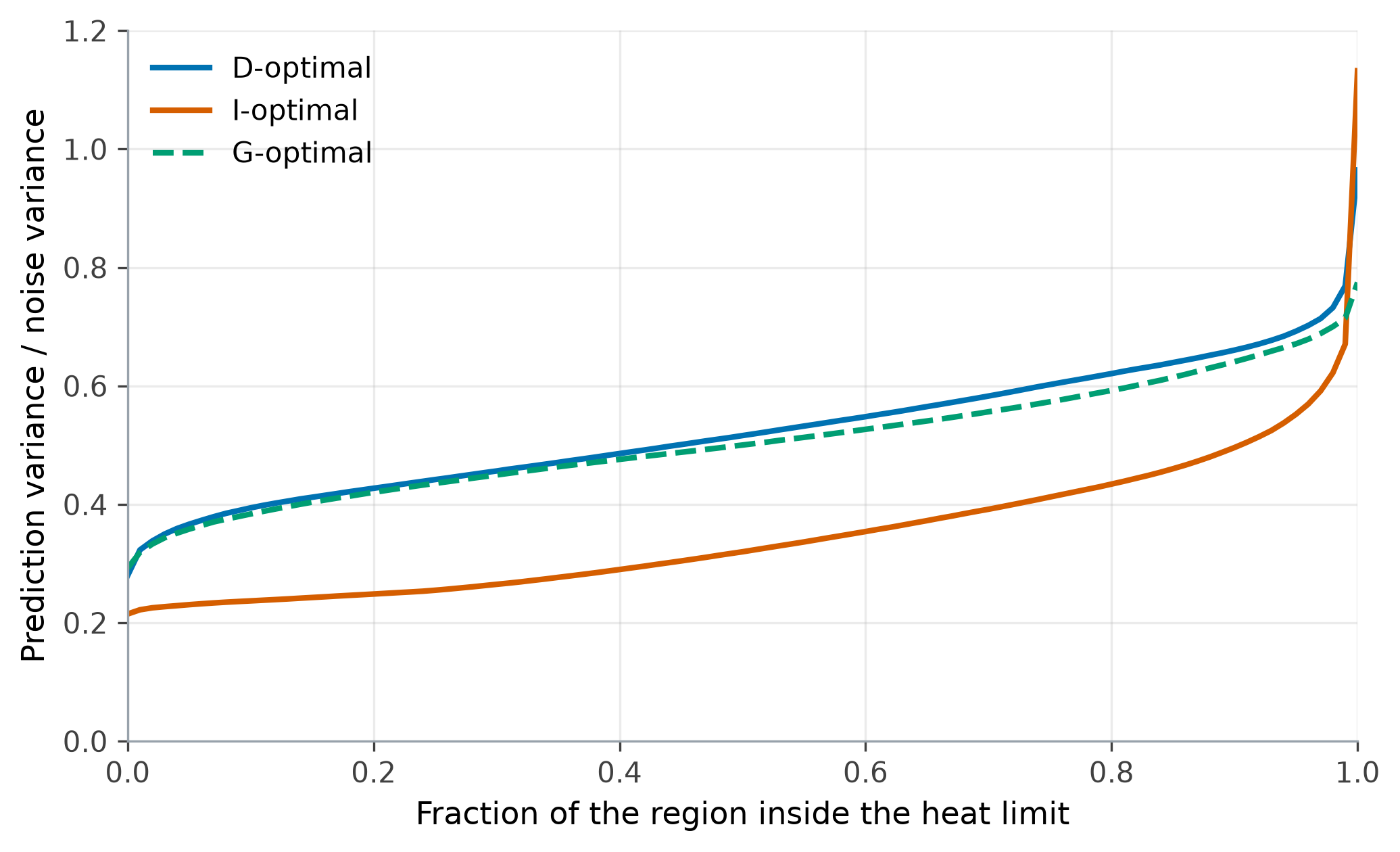
Fraction-of-design-space curves of the three 16-run designs, each judged over the region inside the heat limit. The I-optimal curve is the lowest everywhere except at the far right, where it rises above the other two to the largest maximum: the design accepts a larger worst case, in a small part of the region, for a lower prediction variance everywhere else. The D- and G-optimal curves nearly coincide until the last few percent of the region, where the G-optimal design keeps its maximum lowest.

The plot below sets the face-centred CCD beside the I-optimal design, in the plane of temperature and catalyst loading.

Python, 20 lines

stage2 = designs["i_optimal"]
shapes = {10: "triangle-down-open", 25: "circle-open", 40: "triangle-up-open"}
dodge = {10: -1.5, 25: 0.0, 40: 1.5}   # degC, so runs sharing T and C stay visible
fig = make_subplots(rows=1, cols=2, shared_yaxes=True,
                    subplot_titles=["Face-centred CCD, 17 runs", "I-optimal design, 16 runs"])
for col, design in enumerate([ccd, stage2], start=1):
    runs = design.design_actual
    fig.add_trace(go.Scatter(x=[187.5, 200, 200], y=[2.0, 1.5, 2.0], fill="toself", mode="none",
                             fillcolor="lightgrey", name="beyond the heat limit",
                             showlegend=col == 1), row=1, col=col)
    for minutes, shape in shapes.items():
        at = runs[np.isclose(runs["t"], minutes)]
        colour = np.where(heat(at) > 9.5, "#D55E00", "#0072B2")   # vermilion: beyond the limit
        fig.add_trace(go.Scatter(x=at["T"] + dodge[minutes], y=at["C"], mode="markers",
                                 marker=dict(symbol=shape, size=11, color=colour),
                                 name=f"t = {minutes} min", showlegend=col == 1),
                      row=1, col=col)
    fig.update_xaxes(title_text="Temperature, degC", row=1, col=col)
fig.update_yaxes(title_text="Catalyst loading, mol%", row=1, col=1)
fig.show()

Run in browser

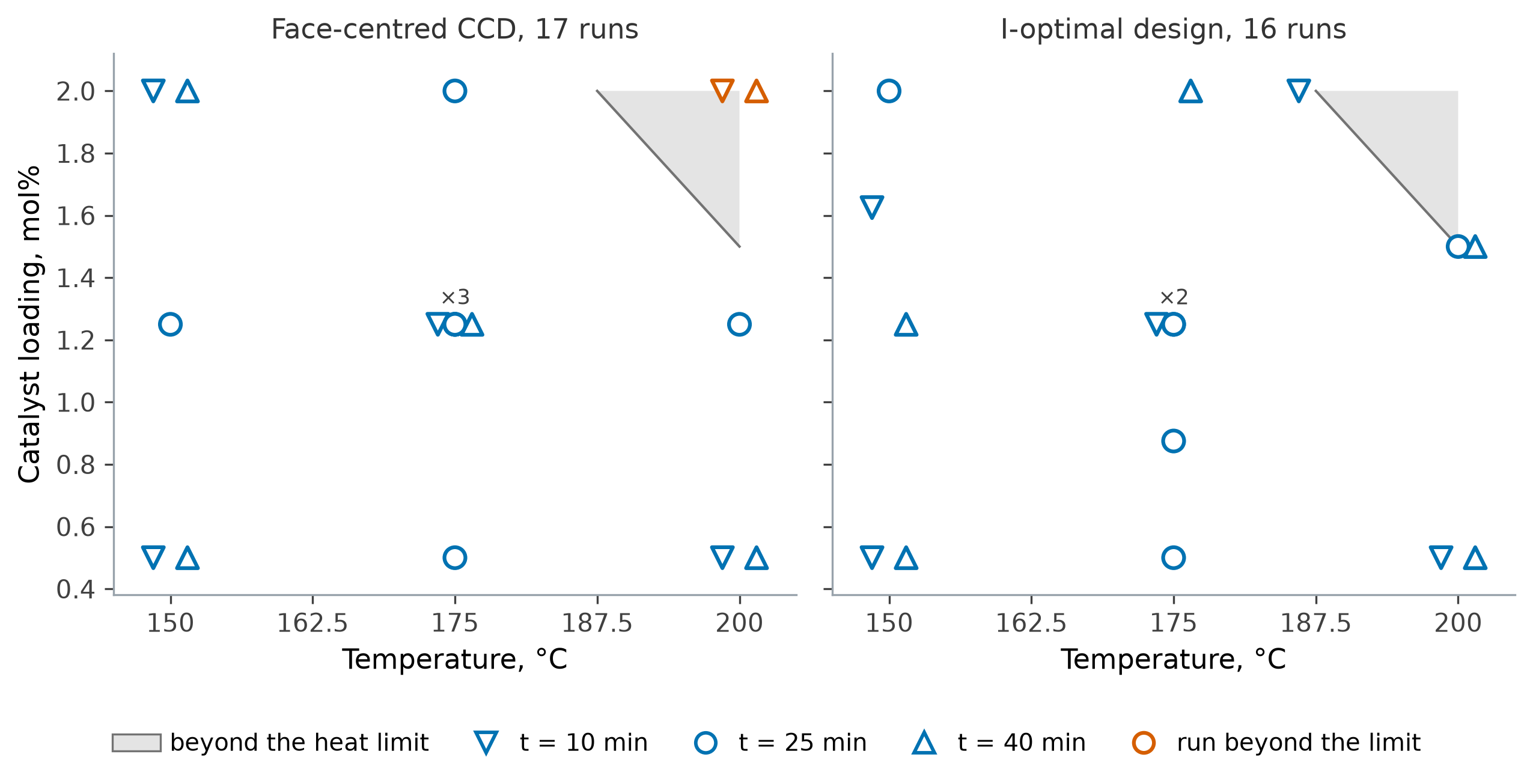
The face-centred CCD (left) and the I-optimal design (right) in the plane of temperature and catalyst loading, with the reaction time shown by the marker shape. Two of the CCD’s cube corners lie beyond the heat limit (vermilion). The I-optimal design keeps every run inside the limit and places three on it, where the next part of the study finds the best settings. Runs at the same temperature and loading are drawn side by side, the shortest reaction time on the left, and repeated runs are counted above their marker.

5.20.5. Choosing the settings inside the limit, and confirming them

When a response improves towards the corner a limit removes, the best allowed settings lie on the limit itself, and an optimiser confined to the allowed region finds them there. The reactor is run at the 16 settings of the I-optimal design and a quadratic model is fitted to each response.

Python, 13 lines

stage2_obs = run_reactor(stage2.design_actual)
datasets, fits = {}, []
for response in ["yield", "impurity"]:
    datasets[response] = stage2.design[["T", "t", "C"]].assign(
        **{response: stage2_obs[response].to_numpy()})
    fit = analyze_experiment(datasets[response], response_column=response, model="quadratic",
                             analysis_type="coefficients")
    fits.append({"response_name": response, "factor_names": ["T", "t", "C"],
                 "coefficients": fit["coefficients"]})
    print(f"{response}: residual standard deviation "
          f"{np.sqrt(fit['model_summary']['mse_residual']):.3f}")
# yield: residual standard deviation 0.526
# impurity: residual standard deviation 0.051

Run in browser

The residual standard deviations are close to the simulator’s noise, 0.5 and 0.05 percentage points, so both quadratic models fit as closely as the noise allows. A real study would make the same comparison with the spread of replicate runs.

The two goals are graded with desirability ramps from 0 to 1: the yield from 0 at 70% to 1 at 80%, and the impurity from 1 at 1.6% to 0 at the 2.0% rejection level. The overall desirability is the geometric mean of the two grades, so settings predicted to reach the rejection level score zero, whatever their yield. Passing the I-optimal design’s region to the optimiser keeps its search inside the heat limit.

Python, 15 lines

goals = [
    {"response": "yield", "goal": "maximize", "low": 70, "high": 80},
    {"response": "impurity", "goal": "minimize", "low": 1.6, "high": 2.0},
]
ranges = {f.name: {"low": f.low, "high": f.high} for f in active}
region = DesignRegion.from_dict(stage2.metadata["region"])
best = optimize_responses(fits, goals, factor_ranges=ranges, region=region)["desirability"]
optimum = pd.DataFrame([best["optimal_actual"]])
setting, predicted = optimum.iloc[0], best["predicted_responses"]
print(f"T {setting['T']:.1f} degC, t {setting['t']:.1f} min, C {setting['C']:.2f} mol%, "
      f"heat {heat(setting):.2f}")
# T 190.1 degC, t 20.4 min, C 1.90 mol%, heat 9.50
print(f"yield {predicted['yield']:.2f}%, impurity {predicted['impurity']:.3f}%, "
      f"overall desirability {best['composite_desirability']:.3f}")
# yield 75.25%, impurity 1.628%, overall desirability 0.699

Run in browser

The recommended settings lie on the heat limit, and the figure below shows why.

Python, 34 lines

def predict(settings):
    """The fitted models' yield and impurity, in %, at settings in actual units."""
    X = quadratic_terms(settings)
    return pd.DataFrame({fit["response_name"]: X @ pd.Series(
        {c["term"]: c["coefficient"] for c in fit["coefficients"]}) for fit in fits})

def desirability(responses):
    """The two ramps of the goals above, and their geometric mean."""
    d = pd.DataFrame({"yield": ((responses["yield"] - 70) / (80 - 70)).clip(0, 1),
                      "impurity": ((2.0 - responses["impurity"]) / (2.0 - 1.6)).clip(0, 1)})
    d["overall"] = np.sqrt(d["yield"] * d["impurity"])
    return d

T_axis, C_axis = np.linspace(150, 200, 51), np.linspace(0.5, 2.0, 51)
TT, CC = np.meshgrid(T_axis, C_axis)
plane = pd.DataFrame({"T": TT.ravel(), "t": setting["t"], "C": CC.ravel()})
times = pd.DataFrame({"T": setting["T"], "t": np.linspace(10, 40, 61), "C": setting["C"]})
along_t = desirability(predict(times))

fig = make_subplots(rows=1, cols=2, subplot_titles=[
    f"Fitted yield, %, at t = {setting['t']:.1f} min", "Desirability along the reaction time"])
fig.add_trace(go.Contour(x=T_axis, y=C_axis, colorbar=dict(x=0.45),
                         z=predict(plane)["yield"].to_numpy().reshape(TT.shape)), row=1, col=1)
fig.add_trace(go.Scatter(x=[187.5, 200, 200], y=[2.0, 1.5, 2.0], fill="toself", mode="none",
                         fillcolor="lightgrey", name="beyond the heat limit"), row=1, col=1)
fig.add_trace(go.Scatter(x=[setting["T"]], y=[setting["C"]], mode="markers",
                         marker=dict(symbol="star", size=16), name="recommended"), row=1, col=1)
for column in ["yield", "impurity", "overall"]:
    fig.add_trace(go.Scatter(x=times["t"], y=along_t[column], name=f"{column} desirability"),
                  row=1, col=2)
fig.update_xaxes(title_text="Temperature, degC", row=1, col=1)
fig.update_yaxes(title_text="Catalyst loading, mol%", row=1, col=1)
fig.update_xaxes(title_text="Reaction time, min", row=1, col=2)
fig.show()

Run in browser

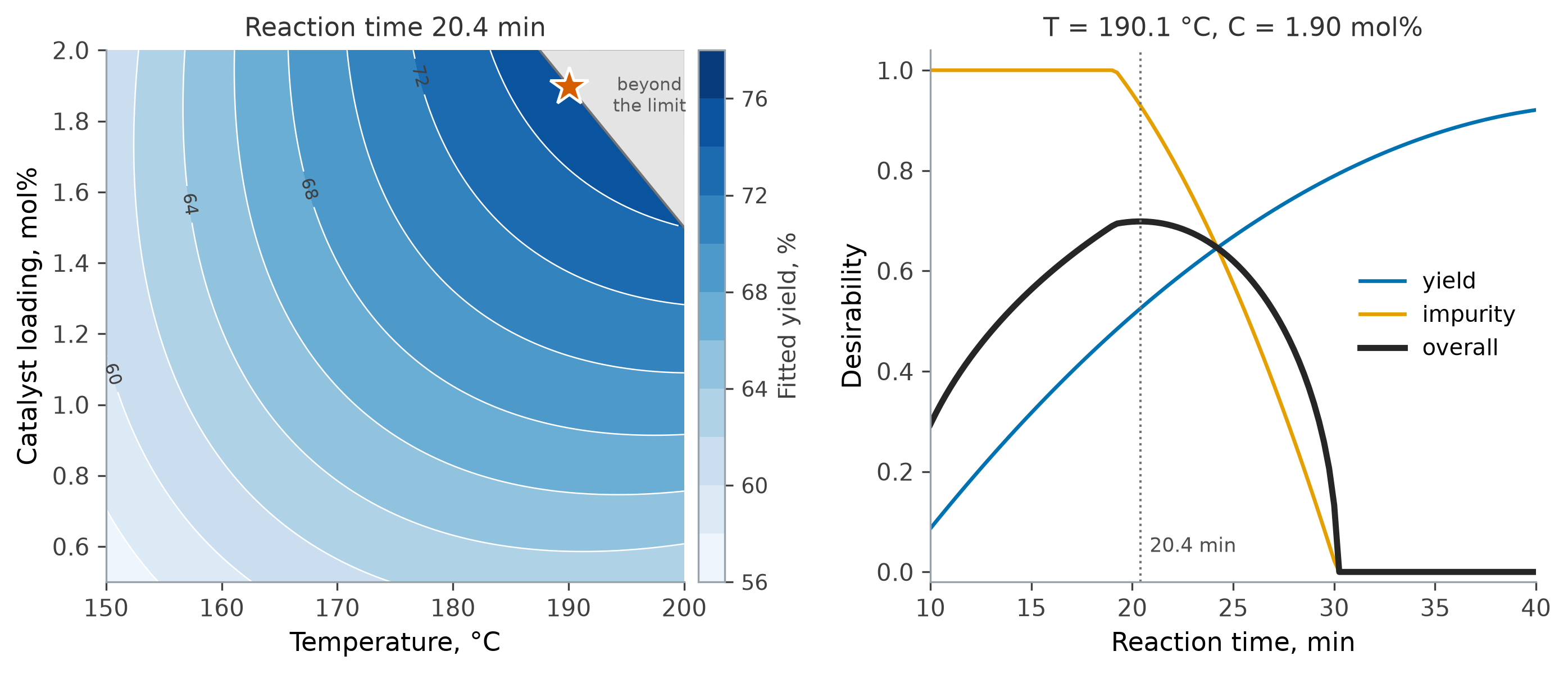
Why the study recommends these settings. Left: the fitted yield at the recommended reaction time, drawn where the heat limit allows. It rises towards the grey corner beyond the limit, so the best allowed settings, the star, lie on the limit. Right: along the reaction time, at the recommended temperature and loading, a longer reaction raises the yield desirability and lowers the impurity desirability. Their geometric mean, the overall desirability, peaks where the two balance.

A recommended setting is a prediction, and confirmation runs test it where it will be used. Three batches are run at the recommended settings, and each observation is compared with the 95% prediction interval for a single new run: the interval that covers one future batch rather than the long-run mean (How well is the optimum known?).

Python, 11 lines

confirm = run_reactor(pd.concat([optimum] * 3, ignore_index=True))
for response in ["yield", "impurity"]:
    check = analyze_experiment(datasets[response], response_column=response, model="quadratic",
                               analysis_type="confirmation_test",
                               new_points=pd.DataFrame([best["optimal_coded"]] * 3),
                               observed_at_new=confirm[response].tolist())["confirmation_test"]
    low, high = check["results"][0]["pi_low"], check["results"][0]["pi_high"]
    observed = ", ".join(f"{value:.2f}" for value in confirm[response])
    print(f"{response}: observed {observed}; 95% prediction interval {low:.2f} to {high:.2f}")
# yield: observed 75.31, 75.74, 75.00; 95% prediction interval 73.65 to 76.85
# impurity: observed 1.69, 1.59, 1.65; 95% prediction interval 1.47 to 1.78

Run in browser

All six observations fall inside their intervals, so the models predict batches at the recommended settings as well as their fit to the 16 runs implied.

5.20.6. How close the study comes to the best settings

The 36 runs found settings with 99.2% of the best overall desirability the reactor allows inside the heat limit. The best settings come from giving the simulator’s true models, rather than the fitted ones, to the same optimiser with the same goals and region; both sets of settings are then scored on the true responses.

Python, 16 lines

true_fits = [{"response_name": r, "factor_names": ["T", "t", "C"],
              "coefficients": [{"term": term, "coefficient": b} for term, b in model.items()]}
             for r, model in TRUE_MODELS.items()]
truth = optimize_responses(true_fits, goals, factor_ranges=ranges,
                           region=region)["desirability"]

both = pd.concat([optimum, pd.DataFrame([truth["optimal_actual"]])], ignore_index=True)
scored = pd.concat([both, true_response(both), desirability(true_response(both))["overall"]],
                   axis=1)
for label, row in zip(["found by the study", "true optimum"], scored.to_dict("records")):
    print(f"{label}: T {row['T']:.1f}, t {row['t']:.1f}, C {row['C']:.2f}; "
          f"yield {row['yield']:.2f}, impurity {row['impurity']:.3f}, D {row['overall']:.3f}")
# found by the study: T 190.1, t 20.4, C 1.90; yield 75.61, impurity 1.682, D 0.668
# true optimum: T 187.6, t 20.3, C 2.00; yield 75.54, impurity 1.672, D 0.674
print(f"{scored['overall'].iloc[0] / scored['overall'].iloc[1]:.1%}")
# 99.2%

Run in browser

Both sets of settings lie on the heat limit, a few degrees apart along it, and the true yields and impurities they give differ by far less than the batch-to-batch noise. For someone running the reactor, the two recipes could not be told apart from a handful of batches.