5.17. A worked OMARS study: four factors on a fed-batch bioreactor

The OMARS trade-off table says what each run count makes estimable, and the staged analysis says how to fit the result. Neither says what the runs are worth. This section runs a study end to end on a process whose true behaviour is known, so the answer can be given in the units a team budgets in: grams per litre of product, and weeks of bioreactor time.

The process is a cell-culture bioreactor like the one met in Fractional factorial designs, where a run takes ten days and a full factorial in five factors “would take almost a year … if parallel reactors are not available”. Parallel reactors are now the normal way such studies are run. A multi-parallel mini-bioreactor system such as the Sartorius Ambr 250 high throughput holds 12 or 24 single-use vessels of 100 to 250 mL under individual control. The batches inoculated and run together on such a system form one parallel run. On a 24-vessel system, thirty batches need two parallel runs: about three and a half weeks of bioreactor time, or six to seven weeks from thawing the cell bank to the last titer result once the seed train and the assays are counted. That is the calendar the run counts below are measured against.

The simulator is process_improve.simulation.batch, a ten-day fed-batch bioreactor with growth following the cardinal temperature and pH model of Rosso et al. (1995), production following Luedeking and Piret (1959), an oxygen-transfer ceiling, hypothermic growth arrest, and substrate-coupled production. Its kinetics are fixed and documented, so the true optimum is computable and every recovered result can be scored against it. The noise the study faces is the simulator’s own, with its within-batch disturbance set to 0.7 of the default.

5.17.1. The process and the question

The current recipe grows the culture at 36.8 °C, starts a temperature downshift on day 2.75 that takes 1.5 days to reach a production hold at 30 °C, holds pH at 7.1 throughout, and feeds at a constant 0.055 L/day per litre of starting volume. The downshift is a programmed ramp; many processes step the setpoint instead. The feed runs from inoculation, so over ten days it adds 40% to 70% of the starting volume across the range studied; vessels started at 140 mL finish at no more than 238 mL, within the 250 mL working limit. Titer, the product concentration at harvest, runs 7 to 8 g/L, which is typical of an intensified fed-batch process seeded at a high cell density. The team wants to know whether the hold temperature, the timing of the downshift, the pH and the feed rate should move, and by how much.

Four factors, one response. Their ranges are what a process engineer would choose around a running recipe, and the centre of each is the current setting:

Factor	Low	Centre	High
Production hold temperature, °C	28.5	30.0	31.5
Temperature downshift, day	2.0	2.75	3.5
pH setpoint	6.9	7.1	7.3
Feed rate, L/day per litre	0.040	0.055	0.070

Every figure in this section is reproducible with process_improve. Each block imports what it needs and reuses variables from the blocks before it, so paste them in order.

Python, 39 lines

import dataclasses
import itertools

import numpy as np
import pandas as pd
from scipy import optimize, stats

from process_improve.experiments import Factor, analyze_omars, generate_omars
from process_improve.simulation import BioreactorConfig, BioreactorSimulator

factors = [
    Factor(name="hold_temp", low=28.5, high=31.5),    # production hold temperature, degC
    Factor(name="shift_day", low=2.0, high=3.5),      # day the downshift starts
    Factor(name="pH", low=6.9, high=7.3),
    Factor(name="feed_rate", low=0.040, high=0.070),  # L/day per litre of starting volume
]
names = [f.name for f in factors]
GROWTH_TEMP, RAMP_DAYS = 36.8, 1.5

# Within-batch disturbance at 0.7 of the simulator's default: a replicate CV near 3%.
config = dataclasses.replace(BioreactorConfig(), within_batch_scale=0.7)

def recipe(cfg, hold_temp, shift_day, pH):
    """The setpoint schedule for one batch: warm growth, a ramp, then the cold hold."""
    days = cfg.interval_start_days
    fraction = np.clip((days - shift_day) / RAMP_DAYS, 0.0, 1.0)
    temperature = GROWTH_TEMP - (GROWTH_TEMP - hold_temp) * fraction
    return pd.DataFrame({"pH": np.full_like(days, pH), "temperature": temperature},
                        index=pd.Index(days, name="day"))

def run_batch(cfg, hold_temp, shift_day, pH, feed_rate, random_state):
    """Final titer, in g/L, of one batch at these settings."""
    sim = BioreactorSimulator(dataclasses.replace(cfg, feed_rate=feed_rate))
    return sim.simulate_batch(trajectory=recipe(cfg, hold_temp, shift_day, pH),
                              random_state=random_state).titer

current = {"hold_temp": 30.0, "shift_day": 2.75, "pH": 7.1, "feed_rate": 0.055}
reps = np.array([run_batch(config, **current, random_state=s) for s in range(20)])
print(f"{reps.mean():#.4g} {reps.std(ddof=1):#.4g}")   # 7.477 0.2308, a CV of 3.1%

Run in browser

Twenty replicate batches at the current recipe give 7.477 g/L with a standard deviation of 0.2308 g/L, a coefficient of variation of 3.1%. That is the noise every effect below is measured against. The response is analysed as log titer, because the kinetics are multiplicative: a change that scales titer by a fixed fraction becomes a fixed difference on the log scale.

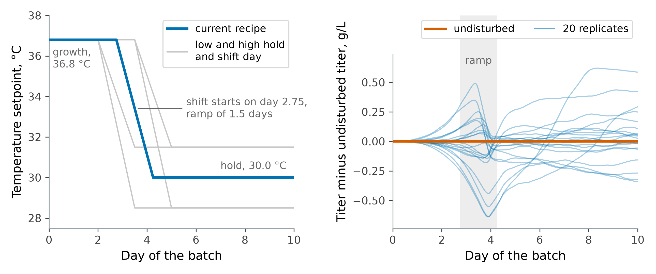
The current recipe, and what one run of it gives. Left: the temperature setpoint through the ten-day batch, with all four combinations of the low and high hold temperature and downshift day in grey; pH is held at 7.1 throughout. Right: for each of the twenty replicate batches, each with its own disturbance draw, the titer minus that of the same batch with no disturbance. The departures build through the growth phase and the ramp, and their spread at harvest is the 0.2308 g/L standard deviation the study measures its effects against.

5.17.2. Choosing the run count

The four-factor column of the trade-off table offers Quad from 10 runs and Full from 21, with the Box-Behnken design at 27. The team has no reason to expect the interactions to be absent, and the downshift timing and hold temperature are the sort of pair that plausibly interact, so the study needs Full: every two-factor interaction in the model. That leaves any size from 21 runs, the frontier, upwards. The upcoming section What the run count buys compares sizes from 13 to 31 runs. For now we study 27 runs, the size of the Box-Behnken design, and add three centre runs, for thirty batches in two parallel runs.

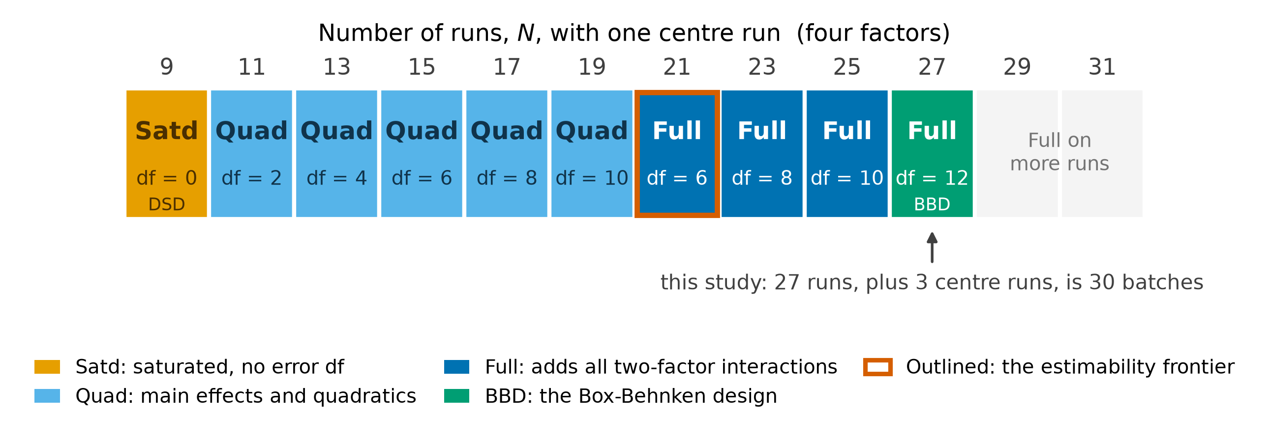
The four-factor column of the OMARS trade-off table, at every odd run count from the nine-run definitive screening design to 31 runs. Each cell names the largest model that run count makes estimable and the error degrees of freedom left to test it. The outlined cell at 21 runs is the estimability frontier, the first at which every two-factor interaction can be estimated. The Box-Behnken design at 27 runs closes the column, since every larger run count repeats Full with more degrees of freedom.

5.17.3. Building the campaign

Python, 3 lines

design = generate_omars(factors, n_runs=27, model="full_second_order", random_state=42)
coded = design.design[names].to_numpy(float)
print(design.metadata["model_rank"], design.metadata["expected_error_df"])   # 15 12

Run in browser

The 27 runs are thirteen half-rows, their thirteen mirror images, and one centre run. The two parallel runs are weeks apart, so anything that differs between them, a new lot of feed medium in this study, moves the titer of every batch in the second parallel run. Each parallel run is therefore a block, a group of runs that share conditions the study does not control, and the design is run in two blocks. The shift between them must not be confused with a factor effect, and a foldover makes that easy to arrange: keep each half-row with its mirror image in the same block, and every main effect sums to zero within each block, whichever way the pairs are divided.

Python, 10 lines

is_centre = np.all(coded == 0, axis=1)
rows = [i for i in range(len(coded)) if not is_centre[i]]
pairs, seen = [], set()
for i in rows:
    if i in seen:
        continue
    j = next(k for k in rows if k not in seen and k != i and np.allclose(coded[k], -coded[i]))
    pairs.append((i, j))
    seen.update((i, j))
print(len(pairs), int(is_centre.sum()))   # 13 mirror pairs, 1 centre run

Run in browser

The second-order columns do not sum to zero within a block, so the split of the thirteen pairs into seven and six is chosen to keep the block indicator as nearly uncorrelated with the quadratics and interactions as it can be. There are 1716 ways to choose seven pairs from thirteen; all are tried.

Python, 21 lines

def second_order_columns(C):
    cols = [C[:, i] ** 2 for i in range(C.shape[1])]
    cols += [C[:, i] * C[:, j] for i, j in itertools.combinations(range(C.shape[1]), 2)]
    return np.column_stack(cols)

so = second_order_columns(coded)
keep = ~is_centre
best_split, best_r = None, np.inf
for chosen in itertools.combinations(range(len(pairs)), 7):
    block = np.full(len(coded), -1.0)
    for p in chosen:
        block[list(pairs[p])] = 1.0
    r = max(abs(np.corrcoef(block[keep], so[keep, c])[0, 1])
            for c in range(so.shape[1]) if so[keep, c].std() > 0)
    if r < best_r:
        best_split, best_r = chosen, r
block = np.full(len(coded), -1.0)
for p in best_split:
    block[list(pairs[p])] = 1.0
# the largest |r| between the block indicator and any second-order column
print(f"{best_r:#.4g}")   # 0.2829

Run in browser

Three centre runs are added so that each parallel run carries two, placed about a third and two thirds of the way through its run order rather than together. The run order within a parallel run is otherwise random.

Python, 21 lines

rng = np.random.default_rng(7)
plan = pd.DataFrame(coded, columns=names)
plan["parallel_run"] = np.where(block > 0, 1, 2)
plan.loc[is_centre, "parallel_run"] = 1
extra = pd.DataFrame(np.zeros((3, 4)), columns=names)
extra["parallel_run"] = [1, 2, 2]
plan = pd.concat([plan, extra], ignore_index=True)

order = []
for c in (1, 2):
    idx = plan.index[plan["parallel_run"] == c].to_numpy()
    centres = idx[np.all(plan.loc[idx, names] == 0, axis=1)]
    seq = list(rng.permutation(idx[~np.isin(idx, centres)]))
    for k, cpt in enumerate(centres):
        seq.insert(int(round((k + 1) * len(idx) / (len(centres) + 1))), cpt)
    order.extend(seq)
plan = plan.loc[order].reset_index(drop=True)
plan.index = pd.RangeIndex(1, len(plan) + 1, name="run")
for n, f in zip(names, factors):
    plan[n] = f.low + (plan[n] + 1) / 2 * (f.high - f.low)   # coded to real units
print(plan["parallel_run"].value_counts().sort_index().tolist())   # [16, 14]

Run in browser

The first parallel run holds sixteen batches and the second fourteen. Both fit a 24-vessel system with room to spare.

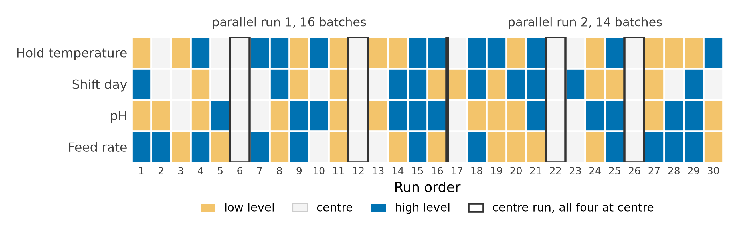
The thirty batches in run order, one column each, with the level of every factor as its fill. The heavy line is the change from the first parallel run to the second, and with it the change of feed-medium lot. The outlined columns, runs 6, 12, 22 and 26, are the centre runs, two in each parallel run and spread through its order. The pair split keeps each mirror pair in one parallel run, which the grid does not show.

5.17.4. Running it

The second parallel run draws on a new lot of feed medium. It passed release testing, but it supports lower productivity, as trace-element differences between lots can. The simulator represents this as 12% less substrate in the feed, which is larger than typical lot-to-lot variation, so that the shift is clear. Nothing else changes between the parallel runs. Each batch gets its own disturbance draw.

Python, 10 lines

lot = {1: config, 2: dataclasses.replace(config, feed_substrate=0.88 * config.feed_substrate)}
seeds = np.random.default_rng(2026).integers(1 << 30, size=len(plan))
plan["titer"] = [run_batch(lot[int(r.parallel_run)], r.hold_temp, r.shift_day, r.pH,
                           r.feed_rate, int(s))
                 for r, s in zip(plan.itertuples(), seeds)]
plan["log_titer"] = np.log(plan["titer"])
print(f"{plan['titer'].min():#.4g} {plan['titer'].max():#.4g}")   # 4.056 9.085

is_cp = np.all(np.isclose(plan[names], list(current.values())), axis=1)
print(plan.loc[is_cp, ["parallel_run", "titer"]])

Run in browser

Output, 6 lines

     parallel_run     titer
run
6               1  7.804948
12              1  7.267075
22              2  6.538538
26              2  6.893483

The titer ranges from 4.056 to 9.085 g/L across the thirty batches, against 7.477 g/L at the current recipe: the region is wide enough that some settings are clearly worse and some clearly better than what the team runs today. The four centre points, at runs 6, 12, 22 and 26, average 7.536 g/L in the first parallel run and 6.716 g/L in the second.

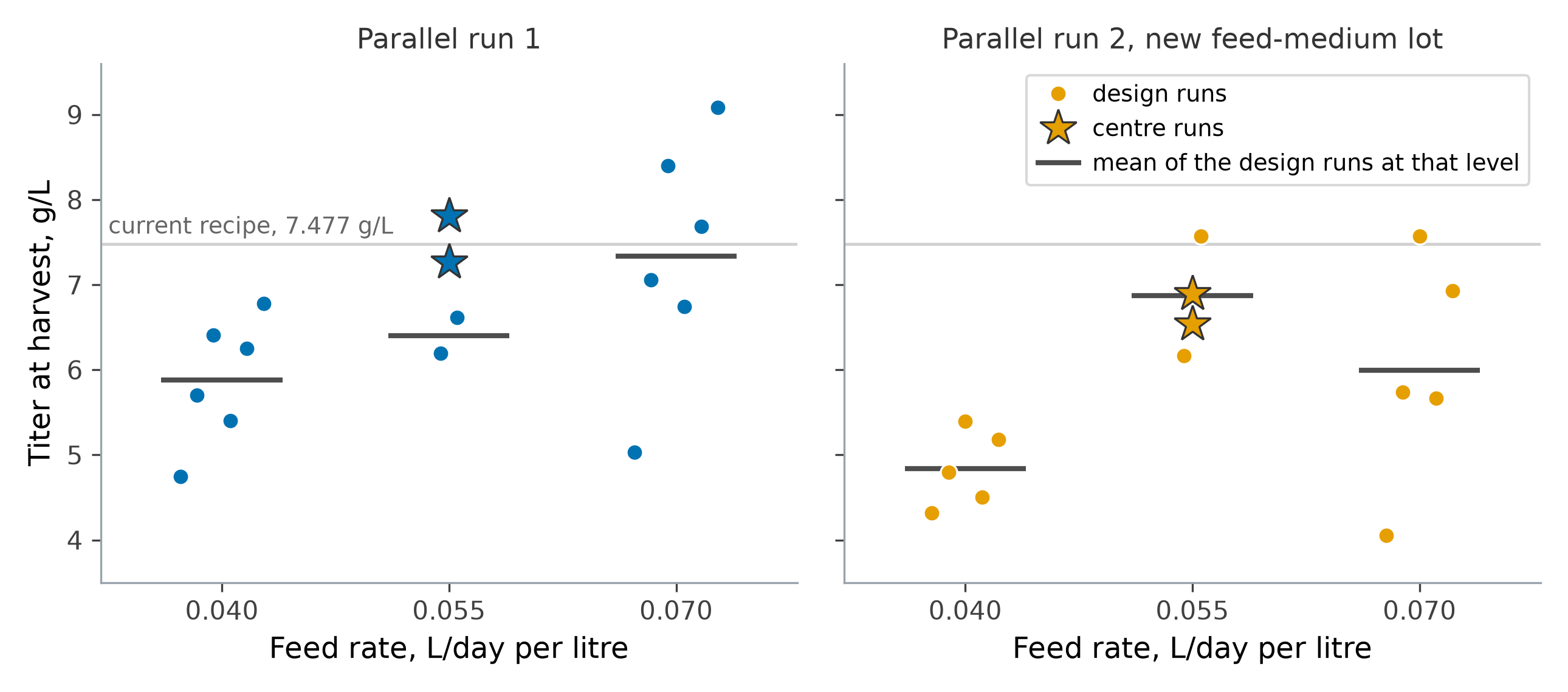
Titer at harvest against the feed rate, one plot per parallel run. The short bars are the mean of the design runs at each feed level; the other three factors vary within each group, which is most of the scatter around the bars. The centre runs, drawn as stars, are the only batches at identical settings in both parallel runs, and their means differ by 0.820 g/L. The grey line is the mean of the twenty replicate batches at the current recipe, 7.477 g/L.

5.17.5. The shift between the parallel runs

The centre points suggest the second parallel run gave lower titers, but four points on two degrees of freedom cannot say so with any confidence. The design as a whole can. A least-squares fit of log titer on a parallel-run indicator and the four main effects estimates the shift from all thirty runs, and because whole mirror pairs were kept together, the main effects and the parallel-run indicator are exactly orthogonal, so neither steals from the other.

Python, 16 lines

C = np.column_stack([(plan[n] - f.low) / (f.high - f.low) * 2 - 1
                     for n, f in zip(names, factors)])
second_run = np.where(plan["parallel_run"] == 2, 1.0, 0.0)
X = np.column_stack([np.ones(len(plan)), second_run, C])
b = np.linalg.lstsq(X, plan["log_titer"], rcond=None)[0]
resid = plan["log_titer"] - X @ b
df = len(plan) - X.shape[1]
se = np.sqrt(resid @ resid / df * np.linalg.inv(X.T @ X)[1, 1])
print(f"{b[1]:#.4g} {se:#.4g} {b[1] / se:#.4g} on {df} df")   # -0.1470 0.06611 -2.223 on 24 df

cp = plan[is_cp]
t_cp = stats.ttest_ind(cp.loc[cp.parallel_run == 2, "log_titer"],
                       cp.loc[cp.parallel_run == 1, "log_titer"])
print(f"{t_cp.statistic:#.4g} {t_cp.pvalue:#.4g}")   # -2.587 0.1226

plan["log_titer_adj"] = plan["log_titer"] - b[1] * second_run

Run in browser

The second parallel run gave titers 0.1470 log units lower, a titer 13.7% below the first, with a standard error of 0.06611: a t of 2.223 on 24 degrees of freedom. The four centre points on their own give a similar t, 2.587, and a p-value of 0.12, because they have two degrees of freedom to judge it on. The signal is the same size in both; only the design has the degrees of freedom to call it. The shift is subtracted from the second parallel run’s responses, and the rest of the analysis works on the adjusted values.

Subtracting one number treats the lot change as the same at every setting. The simulator, with every disturbance switched off, shows what it really was at each of the thirty settings:

Python, 7 lines

quiet = dataclasses.replace(config, ic_scale=0.0, within_batch_scale=0.0, noise_scale=0.0)
weak = dataclasses.replace(quiet, feed_substrate=0.88 * quiet.feed_substrate)
lot_effect = np.array([np.log(run_batch(weak, *s, random_state=0)
                              / run_batch(quiet, *s, random_state=0))
                       for s in plan[names].itertuples(index=False)])
print(f"{lot_effect.min():#.4g} {lot_effect.max():#.4g} {lot_effect.mean():#.4g}")
# -0.1302 -0.007656 -0.09574

Run in browser

The weaker lot lowered log titer by between 0.007656 and 0.1302, depending on the settings. The estimate of 0.1470 is within one standard error of the average of 0.09574, and the part of the lot effect that varies with the settings stays in the residuals of the analysis.

This is the practical reason to build a block into a design rather than to hope a few replicates will reveal one afterwards. Keeping each mirror pair within one block is the scheme Jones and Nachtsheim (2016) proposed for definitive screening designs, and it makes the blocks orthogonal to the main effects. Núñez Ares and Goos (2023), cited in the introduction to OMARS designs, do not keep every pair together: they arrange the blocks to be orthogonal to the main effects and as close as possible to orthogonal to the quadratics and interactions, so those effects are estimated more precisely.

5.17.6. The staged analysis

At thirty runs the full second-order model, fifteen terms, can be fitted in one step, with fifteen degrees of freedom for error. The staged analysis takes a route that also works at the sizes where the full model cannot be fitted at all, and it pools the inactive terms into the error estimate as it goes, which gives it more degrees of freedom to test the second-order terms with.

Python, 9 lines

result = analyze_omars(plan[names], plan["log_titer_adj"],
                       quadratic_heredity="none", interaction_heredity="none")
print(result.active_main_effects)               # ['feed_rate']
print({n: f"{p:#.4g}" for n, p in result.main_effect_p_values.items()})
# {'hold_temp': '0.3976', 'shift_day': '0.3421', 'pH': '0.7741', 'feed_rate': '0.0003220'}
print(result.updated_error_df, f"{result.updated_rmse:#.4g}")   # 18 0.09954
print(f"{result.second_order_overall_p_value:#.4g}")          # 0.0003900
print(result.active_quadratics, result.active_interactions)
# ['hold_temp^2'] ['hold_temp:shift_day', 'hold_temp:feed_rate']

Run in browser

One main effect is declared active, the feed rate. The hold temperature’s linear effect has a p-value of 0.3976, not because the hold temperature does not matter, but because the region straddles its optimum, so the response goes up and then down across the range and the linear term is small. pH, which has no linear effect in this process, has a p-value of 0.7741. The three inactive main effects are pooled into the error, which rises from fifteen to eighteen degrees of freedom.

The gate on the second-order terms then opens, p = 0.00039, and the search selects three of the ten: the hold-temperature quadratic and the interactions of hold temperature with the downshift day and the feed rate.

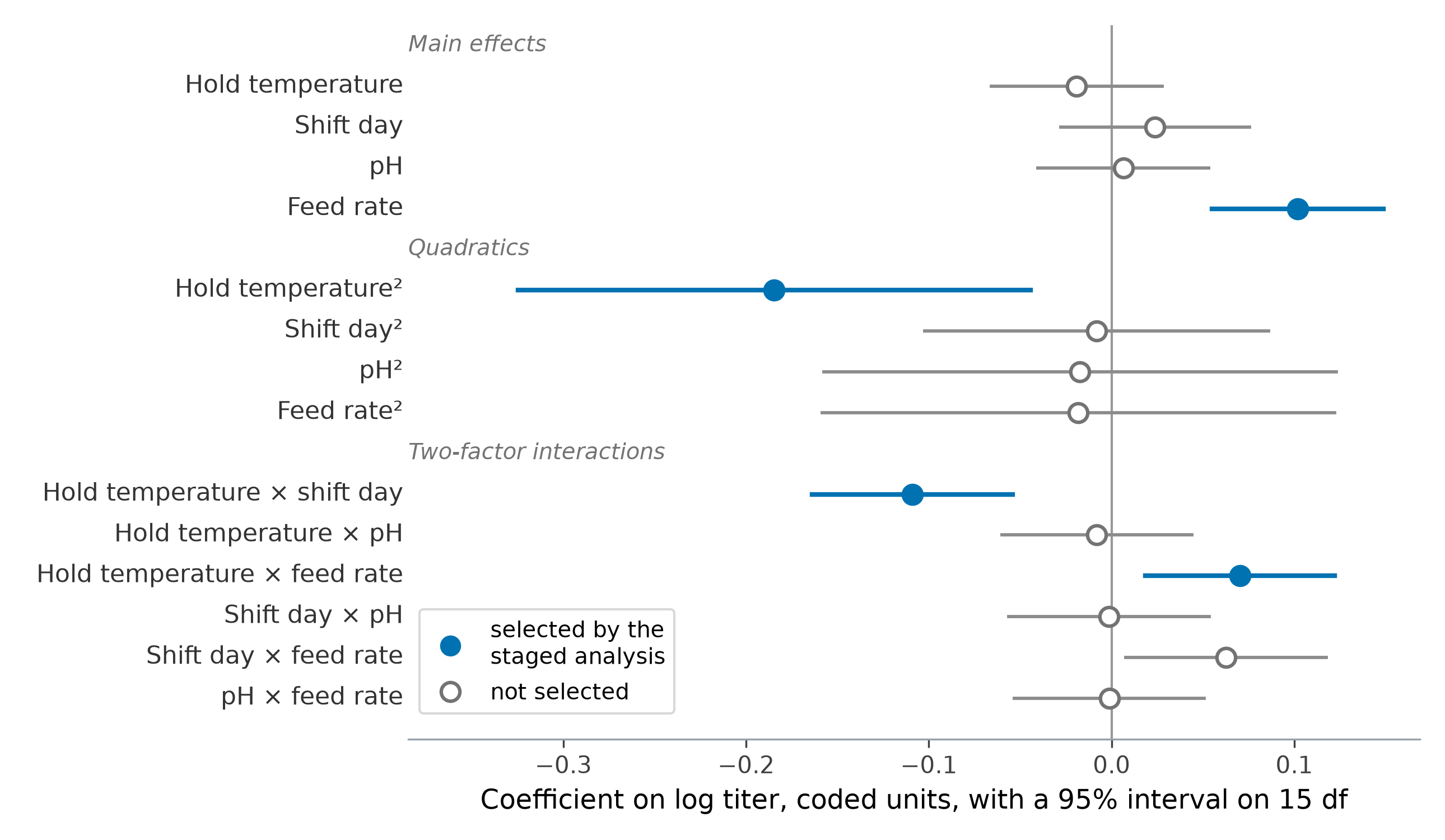
The full second-order model fitted in one step to the thirty adjusted log titers: the fourteen coefficients besides the intercept, with their 95% intervals on fifteen residual degrees of freedom. The filled terms are the four the staged analysis selects, and all four have intervals that exclude zero. A fifth interval also excludes zero, the downshift-day by feed-rate interaction, which the staged analysis does not select; the process does have that interaction, as the model that generated the data lists.

The heredity option changes the result here.

Python, 3 lines

strict = analyze_omars(plan[names], plan["log_titer_adj"],
                       quadratic_heredity="strong", interaction_heredity="strong")
print(strict.active_quadratics, strict.active_interactions)   # ['feed_rate^2'] []

Run in browser

Strong heredity admits a second-order term only if its parent main effects are active. Only the feed rate qualifies, so it offers the feed-rate quadratic alone, and discards the hold-temperature quadratic and both hold-temperature interactions. The hold temperature’s optimum lies near the centre of its range, so its linear effect is small and the rule discards the terms that locate the optimum. Goos et al. (2026) report the opposite case, in which the search without heredity admitted an interaction the process engineers judged spurious, so the staged workflow can be run under both settings and the models compared.

5.17.7. The recommended recipe, against the truth

The selected model has five terms: the intercept, one main effect, one quadratic and two interactions. It is refitted, and its maximum found over the region by refining the best point of a grid, moving only the factors the model mentions: the hold temperature, the downshift day and the feed rate. pH, which the model does not mention, stays at 7.1.

Python, 35 lines

terms = [("m", names.index(m)) for m in result.active_main_effects]
terms += [("q", names.index(q[:-2])) for q in result.active_quadratics]
terms += [("i", tuple(names.index(v) for v in it.split(":")))
          for it in result.active_interactions]

def model_matrix(terms, C):
    C = np.atleast_2d(np.asarray(C, float))
    cols = [np.ones(len(C))]
    for kind, j in terms:
        cols.append(C[:, j] if kind == "m" else C[:, j] ** 2 if kind == "q"
                    else C[:, j[0]] * C[:, j[1]])
    return np.column_stack(cols)

bs = np.linalg.lstsq(model_matrix(terms, C), plan["log_titer_adj"], rcond=None)[0]
moved = sorted({j for k, j in terms if k != "i"} | {v for k, j in terms if k == "i" for v in j})

def predicted(z):
    x = np.zeros(4)
    x[moved] = z
    return -float((model_matrix(terms, x) @ bs).ravel()[0])

def search(f, n):
    """Minimise f over the region: the best of 11 levels per factor, refined within bounds."""
    start = min(itertools.product(np.linspace(-1, 1, 11), repeat=n), key=f)
    return optimize.minimize(f, start, method="L-BFGS-B", bounds=[(-1, 1)] * n)

opt = search(predicted, len(moved))
x_rec = np.zeros(4)
x_rec[moved] = opt.x
decode = lambda x: {n: f.low + (x[i] + 1) / 2 * (f.high - f.low)
                    for i, (n, f) in enumerate(zip(names, factors))}
print({n: f"{v:#.4g}" for n, v in decode(x_rec).items()})
# {'hold_temp': '30.64', 'shift_day': '2.000', 'pH': '7.100', 'feed_rate': '0.07000'}
print(f"{np.exp(-opt.fun):#.4g}")   # predicted titer, g/L
# 8.872

Run in browser

The model recommends a hold at 30.64 °C, the downshift starting on day 2.0, pH left at 7.1 and the feed at 0.070 L/day per litre, and predicts 8.872 g/L there. Two of the three settings it moves are at the edge of the region. The feed rate at its top is what the data say, a strong positive main effect with no feed-rate curvature in the selected model. The downshift day reaches its lower edge through its interaction with hold temperature, with no downshift-day curvature in the model to stop it. A recommendation on a boundary is the model saying it does not know the shape of the response in that direction.

That the selected model has no feed-rate curvature is partly a property of the simulator. From about day 4 its culture runs short of substrate:

Python, 6 lines

sim = BioreactorSimulator(dataclasses.replace(quiet, feed_rate=current["feed_rate"]))
states = sim.simulate_batch(trajectory=recipe(quiet, current["hold_temp"], current["shift_day"],
                                              current["pH"]), random_state=0).states
substrate = states.loc[4:, "substrate"]
print(f"{states['substrate'].iloc[0]:#.4g} {substrate.min():#.4g} {substrate.max():#.4g}")
# 5.000 0.1360 0.2648

Run in browser

That is against 5.000 g/L at inoculation, so within this range more feed raises the titer. A process whose glucose is controlled at a setpoint would usually show curvature in the feed rate.

The simulator settles what the data could not. With every disturbance switched off, the true titer at any recipe is a single number.

Python, 27 lines

truth = lambda x: run_batch(quiet, **decode(np.clip(x, -1, 1)), random_state=0)
best = max((optimize.minimize(lambda x: -truth(x), s, method="Powell", bounds=[(-1, 1)] * 4)
            for s in [np.zeros(4), np.array([-1.0, -1, 0, 1]), np.array([-0.5, 0.5, 0, 1])]),
           key=lambda r: -r.fun)
print(f"{truth(np.zeros(4)):#.4g} {truth(x_rec):#.4g} {-best.fun:#.4g}")
# 7.436 8.605 9.442
print({n: f"{v:#.4g}" for n, v in decode(best.x).items()})
# {'hold_temp': '29.52', 'shift_day': '2.624', 'pH': '7.100', 'feed_rate': '0.07000'}

for j in (1, 0):            # the recommendation, with one setting moved to its best
    x_one = x_rec.copy()
    x_one[j] = best.x[j]
    print(names[j], f"{truth(x_one):#.4g}")
# shift_day 8.007
# hold_temp 7.149

# the best hold for the recommended downshift day, and today's recipe with the feed raised
crest = optimize.minimize_scalar(lambda h: -truth(np.r_[h, x_rec[1:]]), bounds=(-1, 1))
print(f"{decode(np.r_[crest.x, x_rec[1:]])['hold_temp']:#.4g} {-crest.fun:#.4g}")
# 30.22 9.157
print(f"{truth(np.r_[0, 0, 0, x_rec[3]]):#.4g}")
# 8.635

for label, x in (("current", np.zeros(4)), ("best", best.x)):   # pH at 6.9, 7.1 and 7.3
    print(label, [f"{truth(np.r_[x[:2], ph, x[3]]):#.4g}" for ph in (-1, 0, 1)])
# current ['7.610', '7.436', '7.610']
# best ['8.044', '9.442', '8.044']

Run in browser

Recipe	True titer, g/L	Gain over current
Current	7.436
Recommended by the study	8.605	1.169
True best in the region	9.442	2.006

The study captured 1.169 g/L of the 2.006 g/L that was available, 58%. The feed rate and pH are right. The downshift day moved in the right direction, earlier than today’s 2.75, but past the true optimum at 2.62 to the edge of the region, and the hold is about 1.1 °C warmer than the best. Raising the feed rate alone, from today’s recipe, gives 8.635 g/L, so the moves in hold temperature and downshift day add nothing to the gain.

The shortfall comes from the hold temperature and the downshift day together, not from either one. Moving only the downshift day to its best value lowers the titer to 8.007 g/L, and moving only the hold temperature lowers it to 7.149 g/L: an early downshift suits a warm hold, so the recommendation sits at the early end of the ridge the interaction draws. The model places it there because it has no downshift-day curvature to say where along the ridge the peak lies.

The recommended hold is also warmer than the crest of that ridge. With the downshift on day 2.0, the true titer peaks at a hold of 30.22 °C, at 9.157 g/L, and falls away more steeply below that hold than above it, as the contour maps below show. A quadratic is symmetric about its peak, so fitted to that lopsided shape it places the peak on the side where the response falls slowly.

Goos et al. (2026) refit a selected model with the main effect of every factor that appears in one of its second-order terms, a convention called model marginality. Here that adds the hold-temperature and downshift-day main effects to the five terms:

Python, 15 lines

marginal = [("m", j) for j in moved] + [t for t in terms if t[0] != "m"]
b_marginal = np.linalg.lstsq(model_matrix(marginal, C), plan["log_titer_adj"], rcond=None)[0]

def predicted_marginal(z):
    x = np.zeros(4)
    x[moved] = z
    return -float((model_matrix(marginal, x) @ b_marginal).ravel()[0])

opt_marginal = search(predicted_marginal, len(moved))
x_marginal = np.zeros(4)
x_marginal[moved] = opt_marginal.x
print({n: f"{v:#.4g}" for n, v in decode(x_marginal).items()})
# {'hold_temp': '29.80', 'shift_day': '3.500', 'pH': '7.100', 'feed_rate': '0.07000'}
print(f"{truth(x_marginal):#.4g}")
# 8.097

Run in browser

The two models agree on the feed rate and pH. They disagree on the downshift day, and with it the hold: the marginal model sends the downshift to the late edge, day 3.5, with the cooler hold a late downshift suits, 29.80 °C, and the true titer there is 8.097 g/L. Neither model has the downshift-day curvature, so the small downshift-day main effect, which the staged analysis did not find significant, decides which edge the recommendation takes. The models agree on the settings the data determine and disagree on the one setting the study did not resolve.

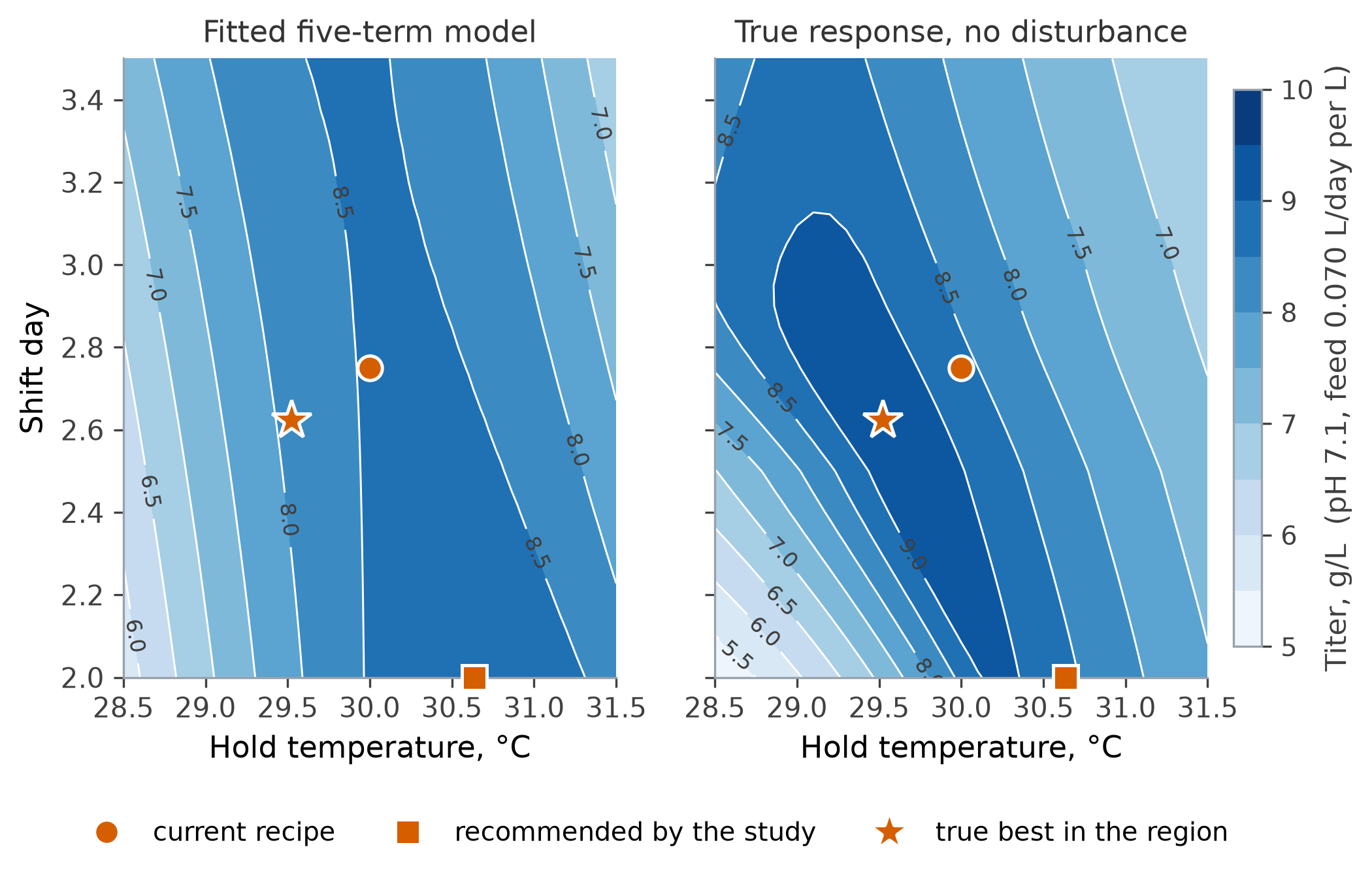
Titer over hold temperature and downshift day, with pH at 7.1 and the feed rate at 0.070 L/day per litre, which is where the recommendation puts both. Left: the five-term model the staged analysis selected, back-transformed from log titer. Right: the simulator with every disturbance switched off. The circle is the current recipe, the square the recipe the study recommends, and the star the true best in the region. The fitted model has no downshift-day curvature, so its best downshift day sits on the edge of the region; the true response has an interior optimum at day 2.62. Along the bottom edge, day 2.0, the true titer rises steeply to its crest near 30.2 °C and falls slowly beyond it, and the square sits on the slow side.

The four centre points supply a pure-error estimate and a test of whether the five-term model is adequate.

Python, 9 lines

rs = plan["log_titer_adj"] - model_matrix(terms, C) @ bs
cp_adj = plan.loc[is_cp, "log_titer_adj"]
pure = ((cp_adj - cp_adj.mean()) ** 2).sum()
df_pe = len(cp_adj) - 1
df_lof = len(plan) - len(bs) - df_pe
F = ((rs @ rs - pure) / df_lof) / (pure / df_pe)
p_lof = 1 - stats.f.cdf(F, df_lof, df_pe)
print(f"{np.sqrt(pure / df_pe):#.4g} {F:#.4g} on ({df_lof}, {df_pe}) df, p = {p_lof:#.4g}")
# 0.04072 6.600 on (22, 3) df, p = 0.07240

Run in browser

The lack-of-fit F is 6.600, with a p-value of 0.0724: not significant at 5%, on three degrees of freedom of pure error, although the model does leave out real effects, as the model that generated the data lists. A team that wanted this test to be more sensitive would run more centre points, or accept, as here, that it is a check rather than a verdict.

5.17.8. How close the study came to the true process

Each setting’s distance from the true optimum, as a percentage of the current recipe, then the fit set against the best second-order approximation of the undisturbed process:

Python, 19 lines

rec, opt, gap = decode(x_rec), decode(best.x), truth(x_rec) + best.fun
print({n: f"{100 * (rec[n] - opt[n]) / current[n]:+.1f}%" for n in names},
      f"titer {100 * gap / truth(np.zeros(4)):+.1f}%")
# {'hold_temp': '+3.7%', 'shift_day': '-22.7%', 'pH': '+0.0%', 'feed_rate': '+0.0%'} titer -11.3%

full = [("m", j) for j in range(4)] + [("q", j) for j in range(4)]
full += [("i", pair) for pair in itertools.combinations(range(4), 2)]
grid = np.array(list(itertools.product(np.linspace(-1, 1, 5), repeat=4)))
b_true = np.linalg.lstsq(model_matrix(full, grid), np.log([truth(x) for x in grid]),
                         rcond=None)[0]
b_fit = np.linalg.lstsq(model_matrix(full, C), plan["log_titer_adj"], rcond=None)[0]
real = np.abs(b_true[1:]) > 1e-6
print(real.sum(), (np.sign(b_fit[1:]) == np.sign(b_true[1:]))[real].sum())   # 10 10
print(f"{b_true[6]:#.4g} {b_fit[6]:#.4g}")   # -0.06627 -0.008206, downshift-day quadratic

opt_true = search(lambda z: -float((model_matrix(full, z) @ b_true)[0]), 4)
share = lambda x: (truth(x) - truth(np.zeros(4))) / (-best.fun - truth(np.zeros(4)))
print(f"{share(x_rec):.0%} {share(opt_true.x):.0%}")   # of the gain available
# 58% 52%

Run in browser

Feed rate and pH are exact; the titer ends 11.3% short of the best. All ten real terms get the right sign, and the five whose intervals exclude zero in the effects figure are all real, so the study declared nothing the process does not have. The miss that moves the recipe is the downshift-day curvature, estimated at an eighth of its size, which sends the downshift to the edge of the region.

Estimating that curvature correctly would not have closed the gap. The best second-order approximation has every term at its true size, yet the recipe at its maximum captures 52% of the gain available, less than the study’s 58%. Within this region the true peak is too narrow and lopsided for a quadratic to place, so the form of the model, more than the data, limits the recommendation.

5.17.9. What the run count buys

Thirty batches in six to seven weeks is a real cost, and the question a team will ask is whether seventeen, or thirteen, would have done, and whether a few more runs would have paid for themselves. The simulator can answer it, because the same study can be rerun at every size with fresh disturbance draws, and each rerun scored the same way: follow the recipe the fitted model recommends, and read the true titer there.

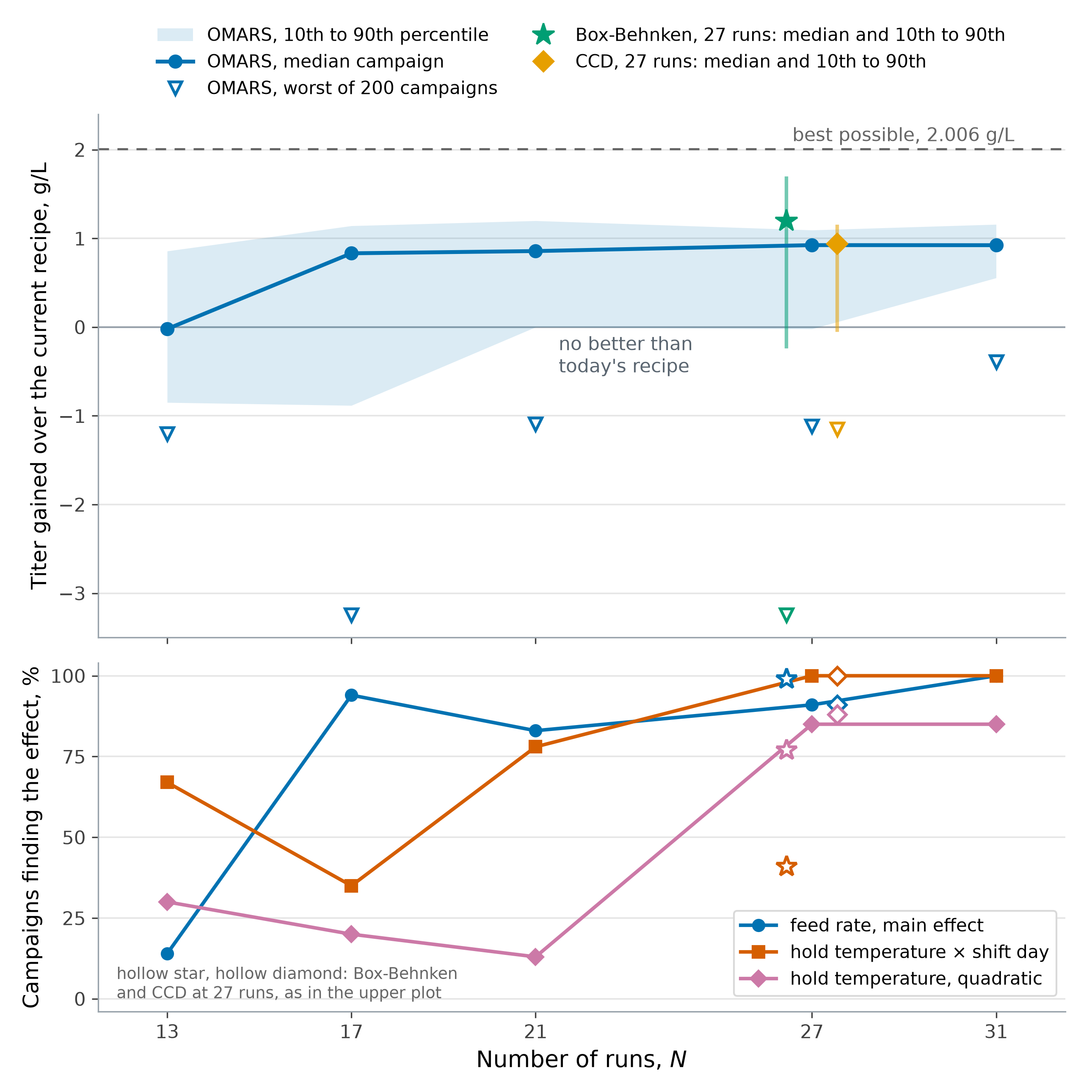
What each design size buys, over two hundred simulated campaigns per design. Upper plot: the line is the median gain in titer at the recipe each campaign recommends, the band runs from the 10th to the 90th percentile, and the marks below are the worst campaign of the two hundred. The dashed line is the 2.006 g/L that was available. Lower plot: the percentage of the same campaigns in which the staged analysis declared each of three of the real effects active. The Box-Behnken and face-centred central composite designs, both 27 runs, are placed beside the 27-run OMARS in both plots.

Gain in titer over the current recipe at each campaign’s recommended recipe, and how often three real effects were declared, over two hundred campaigns per design.

Design	Median gain, g/L	10th percentile, g/L	Worst, g/L	Feed rate, %	Hold x downshift, %	Hold curvature, %
OMARS, 13 runs	-0.02071	-0.8497	-1.201	14	67	30
OMARS, 17 runs	0.8323	-0.8834	-3.246	94	35	20
OMARS, 21 runs	0.8573	0	-1.093	83	78	13
OMARS, 27 runs	0.9244	-0.02071	-1.118	91	100	85
OMARS, 31 runs	0.9236	0.5546	-0.3901	100	100	85
Box-Behnken, 27 runs	1.199	-0.2215	-3.246	99	41	77
Face-centred central composite, 27 runs	0.9403	-0.03423	-1.149	91	100	88

• 13 and 17 runs vary most between the OMARS campaigns. At 13 runs the feed rate is seldom found, so the median campaign gains nothing. At 17 runs it is found, but a design that finds the feed rate without the hold-temperature curvature sends the hold to an edge of the region.

• 21 runs, the frontier, fits the full model but finds the hold-temperature curvature in only 13% of campaigns; its variance factor for that term is the largest of the three Full sizes. Without the curvature, the interaction pairs a cold hold with a late downshift, which gains nearly as much as the median campaign at 27 runs.

• 27 and 31 runs find all three effects in 85% of campaigns or more; the four extra runs raise the lower tail but not the median, which the form of the model limits.

• Box-Behnken has the highest median but finds the interaction in 41% of campaigns; missing it leaves the hold and the downshift at today’s settings, so the median campaign raises only the feed rate, which here does better than moving them.

• Face-centred central composite is close to the 27-run OMARS design throughout.

The variance factor of the hold-temperature quadratic, the diagonal entry of \((\mathbf{X}^T\mathbf{X})^{-1}\) for that term, at the three Full sizes:

Python, 9 lines

def quadratic_variance(n_runs):
    """Variance factor of the hold-temperature quadratic in the full second-order model."""
    levels = generate_omars(factors, n_runs=n_runs, model="full_second_order",
                            random_state=42).design[names].to_numpy(float)
    X = model_matrix(full, levels)
    return np.linalg.inv(X.T @ X)[5, 5]   # column 5 is hold_temp^2

print([f"{quadratic_variance(n):#.4g}" for n in (21, 27, 31)])
# ['0.5367', '0.4215', '0.2446']

Run in browser

5.17.10. The model that generated the data

The simulator’s kinetics are documented in process_improve.simulation.batch. Three features shaped this study:

• Hold temperature: an optimum near 29.5 °C. A warmer hold spends feed on residual growth; a colder one arrests growth before enough biomass is built. Industrial processes more often settle between 31 and 33 °C.

• Downshift day: interacts with the hold. A cold hold favours a late downshift, a warm hold an early one.

• pH: symmetric about 7.1, so no linear effect and no linear-by-linear interaction; its curvature depends on the other factors.

Each batch’s disturbance is an autocorrelated multiplier on growth and production, at 0.7 of the simulator’s default, and the lot change is a 12% cut in feed substrate. From thirty batches the analysis:

• found the feed rate, the hold-temperature curvature, and the hold temperature’s interactions with the downshift day and the feed rate;

• correctly declared no pH main effect;

• missed the downshift-day curvature, which sent the downshift to the edge of the region, the downshift-day by feed-rate interaction, and three smaller terms: the hold-temperature main effect and the curvature in pH and in the feed rate.

5.17.11. How each result traces back to the OMARS properties

Each result of this study follows from a property set out in OMARS designs, and the one miss follows from the model rather than the design. Two checks make that concrete: the feed-rate estimate in the one-step, staged and marginal fits, and the power to detect the true downshift-day curvature, against the error the analysis measures and against the replicate noise alone.

Python, 11 lines

print(f"{b_fit[4]:.4f} {bs[1]:.4f} {b_marginal[3]:.4f}")   # 0.1018 0.1018 0.1018
X_full = model_matrix(full, C)
r = plan["log_titer_adj"] - X_full @ b_fit
df_full = len(r) - X_full.shape[1]
c = np.linalg.inv(X_full.T @ X_full)[6, 6]           # the downshift-day quadratic
f_crit = stats.f.ppf(0.95, 1, df_full)
for sigma in (np.sqrt(r @ r / df_full), np.log(reps).std(ddof=1)):
    nc = (b_true[6] / sigma) ** 2 / c                # noncentrality of the F test
    print(f"{sigma:#.4g} {1 - stats.ncf.cdf(f_crit, 1, df_full, nc):.3f}")
    # 0.1030 0.290
    # 0.03070 0.997

Run in browser

In this study	The property, from 5.16
27 runs fit all fifteen terms with 12 error degrees of freedom	A foldover with one centre run fits the full model from \(k^2 + k + 1 = 21\) runs; 27 runs is the Full df=12 cell (estimability frontier)
Mirror pairs kept in one block leave the block orthogonal to every main effect	A run and its mirror image differ only in sign (mirror-image pairs)
The feed-rate estimate is the same, 0.1018, in all three fits	Main effects are orthogonal to every second-order term (OMARS designs)
Strong heredity drops the hold-temperature terms	Heredity can drop the terms that locate an optimum (analysis)
The 13- and 17-run designs find the hold x downshift interaction less often	In a Quad cell only \(h - k\) interactions, two and four here, can join the model (reading the table)
The downshift-day curvature is missed	Power for a stated effect size (nine measures)

The one miss comes from the model, not the design. A second-order model cannot follow the simulator exactly, so the error the analysis measures, 0.1030 on the log scale, is more than three times the replicate noise, 0.03070. That lowers the power to find the downshift-day curvature from 0.997 to 0.290.

Readings

• Rosso, L., Lobry, J. R., Bajard, S. and Flandrois, J. P.: “Convenient model to describe the combined effects of temperature and pH on microbial growth”, Applied and Environmental Microbiology, 61, 610–616, 1995.

• Luedeking, R. and Piret, E. L.: “A kinetic study of the lactic acid fermentation”, Journal of Biochemical and Microbiological Technology and Engineering, 1, 393–412, 1959.

• Goos, P., Núñez Ares, J., Hameed, M.S.I. and Lanzerath, M.: “An application of a mixed-level OMARS design to a polymerization experiment”, Quality Engineering, 2026. doi:10.1080/08982112.2026.2698477

• Jones, B. and Nachtsheim, C.J.: “Blocking schemes for definitive screening designs”, Technometrics, 58, 74–83, 2016.