
 Download PDF of entire book
5.21. Mixture experiments
Mixture experiments are used to optimize recipes: the factors being varied are the proportions of the ingredients that make up a blend. They arise constantly in fine chemicals, pharmaceuticals, food manufacturing, and polymer processing. As with factorial systems, there are screening and optimization designs for mixtures, but the analysis differs in an important way, because the ingredient proportions are not free to move independently.
5.21.1. The mixture constraint
The defining feature of a mixture experiment is the mixture constraint. If \(x_1, x_2, \ldots, x_q\) are the proportions of the \(q\) ingredients, they must sum to a constant:
(the right-hand side is \(100\) if you prefer percentages, or any positive constant if you mix by weight or volume). The key assumption is that the response depends only on the proportions of the ingredients, not on the total amount of mixture made.
The constraint has one immediate consequence: you cannot change a single ingredient proportion on its own. If you raise \(x_i\), then at least one other proportion \(x_j\) must fall to keep the sum at one. The ingredient proportions therefore cannot be made orthogonal, and their effects cannot be estimated independently, unlike the factors of a factorial design.
Geometrically, the allowed settings form a simplex. For three ingredients this is a triangle, usually drawn as a ternary plot: each vertex is a pure component, each edge is a two-ingredient blend, and the interior holds the full three-ingredient blends. Constraints such as lower or upper bounds on an ingredient cut the simplex down to a smaller region inside it.
5.21.2. How the constraint changes the model
The mixture constraint removes three kinds of term that appear in ordinary response-surface models. Each removal is a case of perfect collinearity: a column of the model matrix \(\mathbf{X}\) equals a linear combination of other columns, so \(\mathbf{X}^T\mathbf{X}\) is singular and the least squares estimator does not exist.
No intercept. If the model has one term per ingredient, those \(q\) columns sum to a column of ones in every row, which is the intercept column. The intercept is therefore redundant and is dropped. This is the same singularity met when a categorical factor is given one dummy per level alongside an intercept.
No pure quadratic terms. Using the constraint, \(x_i = 1 - \sum_{j \ne i} x_j\), so
A pure quadratic \(x_i^2\) is thus a linear combination of the ingredient’s own linear term and its cross-products with the other ingredients. Once the linear and two-factor terms are in the model, the pure quadratics add nothing and must be left out.
No process-variable main effects (when all their blends are present). If a process variable \(z\) (an ordinary factor such as temperature) is crossed with every ingredient, then \(z x_1 + z x_2 + \cdots + z x_q = z\,(x_1 + \cdots + x_q) = z\), so the main effect of \(z\) is redundant with its interactions and is dropped.
5.21.3. Scheffe models
The standard models for a mixture response are the Scheffe models, which build in the removals above. In \(q\) ingredients, the first-order model is
the second-order model adds the two-ingredient blends,
and the special-cubic model adds the three-ingredient blends,
None of these has an intercept or a pure quadratic term. The linear coefficient \(\beta_i\) is the response at the pure component \(x_i = 1\); a positive \(\beta_{ij}\) means the two ingredients blend synergistically (the blend beats the average of the pure components), and a negative one means they work against each other.
The support points of these models sit at recognisable places on the simplex. A second-order Scheffe model in three ingredients has six terms (three linear, three blends), and its natural runs are the three pure-component vertices and the three edge midpoints. The overall centroid is a common extra run, held back to check the fit.
Python, 17 lines
import plotly.graph_objects as go

# Second-order Scheffe support: 3 pure vertices + 3 binary-blend midpoints.
support = [(1, 0, 0), (0, 1, 0), (0, 0, 1),
           (0.5, 0.5, 0), (0.5, 0, 0.5), (0, 0.5, 0.5)]
centroid = [(1 / 3, 1 / 3, 1 / 3)]

fig = go.Figure()
fig.add_trace(go.Scatterternary(
    a=[p[0] for p in support], b=[p[1] for p in support], c=[p[2] for p in support],
    mode="markers", marker=dict(size=12), name="support points"))
fig.add_trace(go.Scatterternary(
    a=[p[0] for p in centroid], b=[p[1] for p in centroid], c=[p[2] for p in centroid],
    mode="markers", marker=dict(size=12, symbol="circle-open"),
    name="centroid (check run)"))
fig.update_layout(ternary=dict(aaxis_title="x1", baxis_title="x2", caxis_title="x3"))
fig.show()

Support points of a second-order Scheffe model in three ingredients: the three pure-component vertices and the three binary-blend edge midpoints, with the overall centroid as an optional check run.
5.21.4. Lower bounds and pseudocomponents
Ingredients often carry lower bounds: a recipe may need at least some of each component. Suppose three ingredients \(a_1, a_2, a_3\) obey \(0.2 \le a_1 \le 0.8\), \(0.2 \le a_2 \le 0.8\), and \(0.0 \le a_3 \le 0.6\). The lower bounds remove a smaller triangle from each corner, but the region that remains is still a simplex of the same shape as the original. The same kind of design is then optimal for the constrained region as for the full one, once we work in pseudocomponents:
where \(L_i\) is the lower bound on ingredient \(i\). The pseudocomponents lie between zero and one and satisfy the mixture constraint. A run at \(x_1 = 100\%\) does not mean a pure first ingredient: with \(\sum L_i = 0.4\) here, it means \(a_1 = 0.8\), \(a_2 = 0.2\), and \(a_3 = 0.0\).
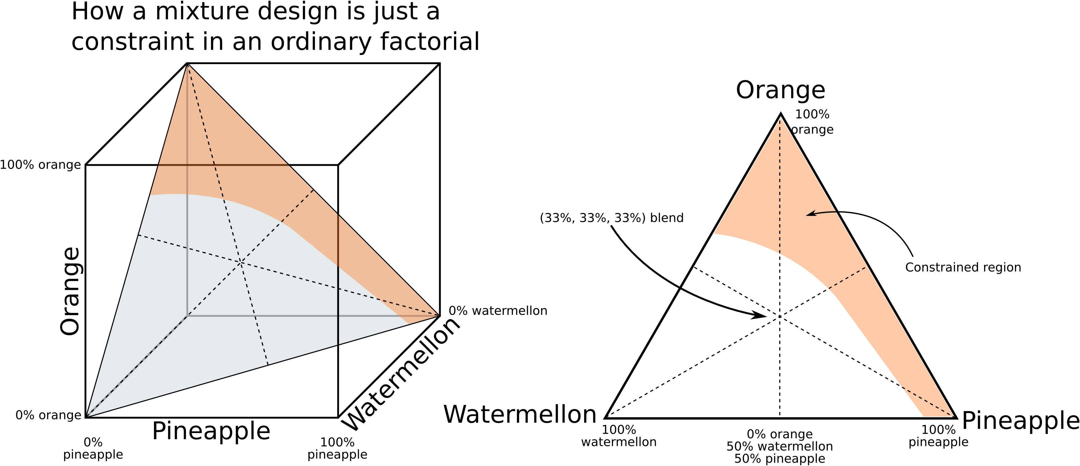
A three-ingredient simplex (left) and a constrained sub-region (right), where the shaded area is infeasible. A D-optimal algorithm places the runs within the remaining region. The example finds a lowest-cost fruit-punch recipe that still meets a taste target, with the shaded region ruling out combinations that are too acidic.
5.21.5. Mixture experiments with process variables
In practice the ingredients are rarely the only factors of interest. Ordinary process variables, such as temperature or mixing speed, often matter too. Such a study is a mixture-process variable experiment, and its model is built by crossing a Scheffe model in the ingredients with a response-surface model in the process variables. Following the removals above, the combined model has no intercept and no process-variable main effects.
The number of parameters grows quickly. For \(q\) ingredients and \(m\) process variables, crossing the quadratic mixture model with a process model of main effects and two-factor interactions needs
parameters, and at least that many runs. For three ingredients and two process variables this is already \(6 \times 4 = 24\). Kowalski, Cornell, and Vining (2000) proposed a more parsimonious second-order model that drops the interactions between the process variables and the non-linear blending terms, which keeps the run count manageable.
One caution: because process variables are often harder to change than a recipe, mixture-process experiments are frequently not fully randomized, but run in a split-plot structure. That changes both the design and the analysis. Split-plot designs are beyond the scope of this chapter; see the references below.
5.21.6. Constructing the design on the simplex
The coordinate-exchange algorithm for ordinary optimal designs changes one coordinate at a time, holding the others fixed. That cannot work on a simplex, because changing one proportion forces the others to move. The mixture version moves each point along the Cox-effect direction: it changes one ingredient while rescaling the others so their pairwise ratios stay fixed and the sum stays at one. When ingredient \(i\) is changed by \(\delta\), each other proportion is updated as
For example, raising \(x_1\) from \(0.30\) to \(0.50\) in the blend \((0.30, 0.30, 0.40)\) rescales the other two to \(0.214\) and \(0.286\), which keep the ratio \(x_2 / x_3 = 0.75\) and still sum to one. Geometrically the point slides along the line from the \(x_1\) vertex through the current point, shown dashed below.
Python, 19 lines
import plotly.graph_objects as go

start = (0.30, 0.30, 0.40)
moved = (0.50, 0.214, 0.286)   # x1 raised by 0.20; x2, x3 rescaled, ratio kept at 0.75
# The Cox-effect direction: the line from the x1 vertex through the point to the
# far edge.
share = start[1] / (start[1] + start[2])
direction = [(1, 0, 0), (0.0, share, 1 - share)]

fig = go.Figure()
fig.add_trace(go.Scatterternary(
    a=[p[0] for p in direction], b=[p[1] for p in direction],
    c=[p[2] for p in direction],
    mode="lines", line=dict(dash="dash"), name="Cox direction"))
fig.add_trace(go.Scatterternary(
    a=[start[0], moved[0]], b=[start[1], moved[1]], c=[start[2], moved[2]],
    mode="markers", marker=dict(size=12), name="x1 raised from 0.30 to 0.50"))
fig.update_layout(ternary=dict(aaxis_title="x1", baxis_title="x2", caxis_title="x3"))
fig.show()

Moving along the Cox-effect direction for ingredient 1, from \((0.30, 0.30, 0.40)\) to \((0.50, 0.214, 0.286)\). The other two proportions shrink but keep their ratio, so the point stays on the line from the \(x_1\) vertex to the opposite edge.
The mixture coordinate-exchange algorithm evaluates the optimality criterion at several points along this direction, within the feasible range set by the bounds and any other constraints, and keeps the best. It repeats over every ingredient of every run until no change improves the design, just as the standard coordinate-exchange does off the simplex.
5.21.7. References
John A. Cornell, Experiments with Mixtures, 3rd edition, Wiley, 2002. ISBN 978-0-471-39367-3.
Wendell F. Smith, Experimental Design for Formulation, SIAM, 2005. ISBN 978-0-898715-80-7.
Scott M. Kowalski, John A. Cornell and G. Geoffrey Vining, “A new model and class of designs for mixture experiments with process variables”, Communications in Statistics: Theory and Methods, 29, 2255-2280, 2000.
Gregory F. Piepel, “Programs for generating extreme vertices and centroids of linearly constrained experimental regions”, Journal of Quality Technology, 20, 125-139, 1988.
Koji Muteki and John F. MacGregor, “Sequential design of mixture experiments for the development of new products”, Journal of Chemometrics, 21, 496-505, 2007.