5.16. OMARS designs: orthogonal minimally aliased response surface designs¶

A definitive screening design is economical but rigid: for a given number of factors it is essentially one design, of one size, with one fixed compromise on interactions. OMARS designs (Orthogonal Minimally Aliased Response Surface designs, Núñez Ares and Goos, 2020) fill the range between a DSD and a central composite design, for when a few more runs can buy better estimates of the interactions.

The defining property generalises the one that makes the DSD work: the main effects are orthogonal to one another and to every second-order effect, quadratics and two-factor interactions alike. The name records this: orthogonal (main effects clean of each other), minimally aliased (main effects clean of the second-order effects), response surface (a full second-order model is the target).

Minimally aliased means zero, not small. The two alias matrices that carry bias into the main effects, one from the interactions and one from the quadratics, are zero by construction; in Judging and comparing designs this appears as main-effect rows of the alias matrix that are exactly zero. Aliasing among the second-order effects remains and varies widely between designs, so choosing the size and choosing within a size are separate questions.

OMARS is a catalogue, not a single design. Núñez Ares and Goos (2020) enumerated it for three to seven factors by integer programming: 7,933 basic designs, or 55,531 with zero to six centre runs added. The spectrum below places them between the DSD and the classical response surface designs.

Most of the catalogue is foldover designs, built like the DSD by stacking a base matrix on its sign-flipped copy. Folding over is sufficient for clean main effects but not necessary: what is required is that all odd design moments through order three are zero. The non-foldover members therefore have equally clean main effects, and can estimate more two-factor interactions jointly than a foldover of the same size (Goos, 2025). Centre runs can be added to any member without disturbing these properties.

The family has been extended to mixed-level designs, with three-level quantitative and two-level categorical factors (Núñez Ares, Schoen and Goos, 2023), and to orthogonally blocked designs (Núñez Ares and Goos, 2023).

Readings

Kiefer, J. and Wolfowitz, J.: “The equivalence of two extremum problems”, Canadian Journal of Mathematics, 12, 363–366, 1960.
Núñez Ares, J. and Goos, P.: “Enumeration and Multicriteria Selection of Orthogonal Minimally Aliased Response Surface Designs”, Technometrics, 62, 21–36, 2020. doi:10.1080/00401706.2018.1549103
Goos, P.: “OMARS designs for factor screening and response surface experimentation in one step: A review”, WIREs Computational Statistics, 17, e70018, 2025. doi:10.1002/wics.70018
Núñez Ares, J., Schoen, E.D. and Goos, P.: “Orthogonal minimally aliased response surface designs for three-level quantitative factors and two-level categorical factors”, Statistica Sinica, 33, 107–126, 2023.
Núñez Ares, J. and Goos, P.: “Blocking OMARS designs and definitive screening designs”, Journal of Quality Technology, 55, 489–509, 2023. doi:10.1080/00224065.2023.2196035

5.16.1. A spectrum from screening to response surface¶

The three families lie on one line. At the economical end, the definitive screening design: the fewest runs, every main effect clean, curvature detectable, the interactions tangled together. In the middle, the larger OMARS designs: more estimable second-order effects, lower correlation among them, and more power. At the rich end, the central composite and Box-Behnken designs, which estimate the full second-order model with little or no aliasing, often with near-rotatable prediction variance. The face-centred central composite and the Box-Behnken designs are themselves among the largest OMARS designs, so the line is one continuous family.

A horizontal axis from few runs to many, with definitive screening designs at the left, OMARS designs in the middle and central composite and Box-Behnken designs at the right. — The three design families on a single axis. Moving from left to right spends more runs and reduces the aliasing among the second-order effects.¶

This suggests a first choice:

Many factors, a tight budget, and a reasonable belief that only a few will matter: a definitive screening design. Screen and glimpse curvature in one economical step.

A handful of factors, and a wish to estimate some interactions and curvature without committing to a full response surface design: a mid-sized OMARS design.

Few factors and a genuine response-surface goal, predicting and optimizing over the region: a central composite or Box-Behnken design, or one of the largest OMARS designs.

Choosing a specific design, even at a fixed budget, uses the measures of Judging and comparing designs: the information matrix, the prediction variance and its fraction-of-design-space plot, the correlations among the effects, and power.

The whole spectrum targets the second-order polynomial. It is the simplest model that can place a maximum, minimum or saddle inside the region; it is linear in its coefficients; and it needs only three levels per factor. Higher-degree polynomials need more levels and tend to oscillate near the edges, so when a quadratic does not fit it is more common to transform the response or fit a different type of model.

5.16.2. A trade-off table for OMARS designs¶

The two-level trade-off table maps a budget of factors and runs onto resolution III, IV or V, the ability to tell main effects apart from interactions.

It is natural to want the same table for OMARS designs, but it is not possible. An OMARS design has its main effects orthogonal to each other and to every second-order term at every size, which is what “orthogonal” and “minimally aliased” in the name record, so resolution is constant and cannot be what the table reports.

What varies with the run count is the model: how much of the second-order model can be fitted at all. That is not the count the parameters suggest.

5.16.2.1. How many runs a second-order model needs¶

The full second-order model in \(k\) factors has an intercept, \(k\) main effects, \(k\) pure quadratics and \(k(k-1)/2\) two-factor interactions:

\[p = 1 + 2k + \frac{k(k-1)}{2}\]

Spending at least \(p\) runs is enough for factorial, central composite, optimal and Box-Behnken designs. For a foldover near the parameter count it is not.

A foldover stacks a half-design \(\mathbf{H}\) of \(h\) runs on its own sign-flipped copy, then adds a centre run:

\[\begin{split}\mathbf{D} = \begin{bmatrix} \mathbf{H} \\ -\mathbf{H} \\ \mathbf{0} \end{bmatrix}, \qquad N = 2h + 1\end{split}\]

A row of \(\mathbf{H}\) and its sign-flipped copy are a mirror-image pair. This construction is behind most of the OMARS catalogue and the definitive screening design, where \(\mathbf{H}\) is a conference matrix.

A mirror-image pair gives identical values in every second-order column, since \((-x_i)^2 = x_i^2\) and \((-x_i)(-x_j) = x_i x_j\). Five runs in two factors show it:

Output, 6 lines

run     x1  x2 |   1   x1²  x2²  x1x2     <- intercept and second-order columns
 H  1   +1  +1 |   1    1    1    +1
 H  2   +1  -1 |   1    1    1    -1
-H  3   -1  -1 |   1    1    1    +1      identical to run 1
-H  4   -1  +1 |   1    1    1    -1      identical to run 2
 0  5    0   0 |   1    0    0     0

Runs 3 and 4 flip sign in the main-effect columns, which is what estimates the main effects, but repeat runs 1 and 2 in the other columns. Those columns therefore see only \(h + 1\) distinct rows, however many runs the foldover contains, and \(h + 1\) rows can separate at most \(h + 1\) terms. Here there are three rows for four columns, and \(x_1^2\) and \(x_2^2\) are the same column.

That one count sets the frontier. The intercept, \(k\) quadratics and \(k(k-1)/2\) interactions are \(1 + k(k+1)/2\) terms, so the full model needs \(h + 1 \ge 1 + k(k+1)/2\), that is

(1)¶\[N = 2h + 1 \; \ge \; k^2 + k + 1\]

The distinct rows must also be linearly independent. A two-level design never manages it, since every non-centre run has \(x_i^2 = 1\); a three-level foldover built for the full model does.

We call this threshold, which has no established name, the estimability frontier: the smallest foldover in which all \(p\) coefficients of the full second-order model can be estimated jointly.

With no centre run or two, \(N\) is even and there are \(N/2\) distinct rows, so an even run count supports the same model as the odd count one below it, with one more spare run. This section assumes one centre run, which reaches each threshold with the fewest runs.

The estimability frontier, against the parameter count it has to clear.¶
Factors, \(k\)	Parameters, \(p\)	Frontier, \(k^2+k+1\)	Shortfall, \(k(k-1)/2\)	Error df at the frontier
3	10	13	3	3
4	15	21	6	6
5	21	31	10	10
6	28	43	15	15
7	36	57	21	21

The last two columns hold the same number: the frontier exceeds \(p\) by \(k(k-1)/2\), exactly the number of two-factor interactions. So for a foldover, more runs than parameters does not make the model estimable; and the smallest design that does, at the frontier, has \(k(k-1)/2\) error degrees of freedom to test it. The four-factor case at nineteen and twenty-one runs:

Python, 22 lines

import itertools
import numpy as np
from process_improve.experiments import Factor, generate_omars

def second_order_matrix(levels):
    """Model matrix of the full second-order model: intercept, main effects,
    pure quadratics, then every two-factor interaction."""
    n_runs, k = levels.shape
    columns = [np.ones(n_runs)]
    columns += [levels[:, i] for i in range(k)]
    columns += [levels[:, i] ** 2 for i in range(k)]
    columns += [levels[:, i] * levels[:, j] for i, j in itertools.combinations(range(k), 2)]
    return np.column_stack(columns)

factors = [Factor(name=c, low=-1, high=1) for c in "ABCD"]
for n_runs, model in ((19, "main_quadratic"), (21, "full_second_order")):
    design = generate_omars(factors, n_runs=n_runs, model=model, random_state=42)
    X = second_order_matrix(design.design[design.factor_names].to_numpy(float))
    print(n_runs, X.shape, np.linalg.matrix_rank(X))

# 19 (19, 15) 13
# 21 (21, 15) 15

At nineteen runs the rank falls two short of the fifteen columns, so the model cannot be fitted despite four spare runs. No foldover rescues it: nineteen runs give ten distinct rows against the eleven intercept and second-order terms, and generate_omars refuses to build one for the full model. Judge estimability from the rank of the model matrix, not from the determinant of the information matrix.

The frontier is a property of the foldover construction, not of OMARS designs as such. The nineteen-run design below, found by computer search, is not a foldover (only six of its eighteen non-centre runs form mirror-image pairs), yet its main effects are orthogonal to each other and to every second-order column, and it estimates the full model. It visits the middle levels of its factors unequally often, which makes it what Goos (2025) calls a non-uniform-precision OMARS design: its main effects are estimated with different precision.

Python, 15 lines

nonfoldover = np.array([
    [-1, -1, 0, -1], [-1, -1, 0, 1], [-1, 0, -1, 1], [-1, 0, 1, -1], [-1, 1, -1, -1],
    [-1, 1, 1, 1], [0, -1, -1, -1], [0, -1, 0, 0], [0, -1, 1, 1], [0, 0, 0, 0],
    [0, 1, -1, 1], [0, 1, 0, 0], [0, 1, 1, -1], [1, -1, -1, 1], [1, -1, 1, -1],
    [1, 0, -1, -1], [1, 0, 1, 1], [1, 1, 0, -1], [1, 1, 0, 1]], dtype=float)
X19 = second_order_matrix(nonfoldover)
G = X19[:, 1:5].T @ X19                       # main effects against every column
G[:, 1:5] -= np.diag(np.diag(G[:, 1:5]))      # ignore each main effect against itself
print(np.abs(G).max(), np.linalg.matrix_rank(X19))   # 0.0 15

for M in (X19, X):                            # X is still the 21-run foldover from above
    c = np.diag(np.linalg.inv(M.T @ M))
    print(len(M), f"{c[5:9].max():#.4g} {c[9:].max():#.4g}")
# 19 10.25 2.000
# 21 0.6800 0.1533

It pays for the two runs it saves: its largest variance factors (the diagonal entries of \((\mathbf{X}^T\mathbf{X})^{-1}\), which multiply \(\sigma^2\) to give a coefficient’s variance) are more than ten times the twenty-one-run foldover’s, for quadratics and interactions alike. The frontier, and the trade-off table built on it, therefore describe foldover designs, which is how generate_omars builds them.

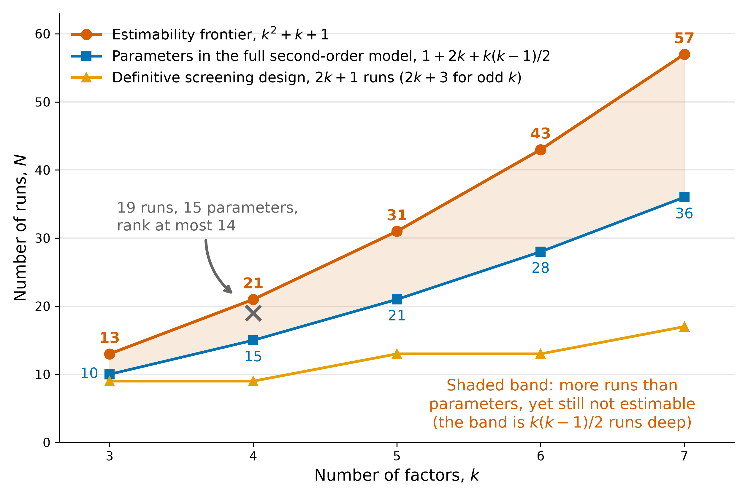
Run count against number of factors from three to seven: the estimability frontier, the parameter count of the full second-order model and the definitive screening design size, with the band between the frontier and the parameter count shaded. — The estimability frontier \(N = k^2 + k + 1\) for a foldover, against the parameter count of the full second-order model and the size of a definitive screening design. In the shaded band, \(k(k-1)/2\) runs deep, a design has more runs than the model has parameters and still cannot estimate it. The marked point is the four-factor case checked in the code.¶

5.16.2.2. Reading the table¶

The frontier defines three capability classes, each tagged with four characters:

Full: \(N \ge k^2 + k + 1\), the estimability frontier. Main effects, pure quadratics and every two-factor interaction are estimable jointly, so one design fits a response surface.
Quad: \(N \ge 2k + 2\). Main effects and pure quadratics are estimable, with degrees of freedom left over to test them. The two-factor interactions are in the design, still orthogonal to the main effects, but not in the fitted model.
Satd: \(N = 2k + 1\). Saturated: the main-effects-plus-quadratics model can be estimated, but nothing is left to estimate \(\sigma^2\), so there are point estimates and no standard errors, tests or power.

The smallest Quad design has \(2k + 2\) runs: the saturated design with a second centre run, which adds one error degree of freedom and no new distinct row.

In a Quad design the interactions cannot all enter the model, but some can. The same count says how many: of the \(h + 1\) distinct rows the intercept and quadratics use \(1 + k\), leaving

(2)¶\[\text{interactions that can be added} \; = \; h - k \; = \; \frac{N-1}{2} - k\]

for an odd \(N\), and the same for the even count one run above it. A seventeen-run design in four factors can carry four of its six interactions, a thirteen-run one only two. The staged analysis of Analysing data from these designs decides which to bring in, and those left out still bias those that come in. Setting \(h - k \ge k(k-1)/2\) recovers the frontier, so Full is exactly where every interaction fits at once.

The tags sort alphabetically in decreasing order of capability. The table and the single-cell report come from process_improve:

Python, 7 lines

from process_improve.experiments import (
    get_omars_trade_off_table_entry,
    omars_trade_off_table,
)

omars_trade_off_table(anchors=True)              # the whole table
get_omars_trade_off_table_entry(17, 4)           # one cell, reported in words

Output, 16 lines

runs  k=3              k=4              k=5              k=6              k=7
-------------------------------------------------------------------------------------------
   Quad df=2 | DSD  Satd df=0 | DSD
  Full 3           Quad 4           Quad df=2 | DSD  Satd df=0 | DSD
  Full 5 | BBD     Quad 6           Quad 4           Quad 2           Satd df=0
                   Quad 8           Quad 6           Quad 4           Quad 2 | DSD
                   Full 6           Quad 10          Quad 8           Quad 6
                   Full 10          Quad 14          Quad 12          Quad 10
                   Full 12 | BBD    Quad 16          Quad 14          Quad 12
                                    Full 10          Quad 18          Quad 16
                                    Full 16          Quad 24          Quad 22
                                    Full 22          Full 15          Quad 28
                                    Full 25 | BBD    Full 18          Quad 31
                                                     Full 26 | BBD    Quad 39
                                                                      Full 21
                                                                      Full 26 | BBD

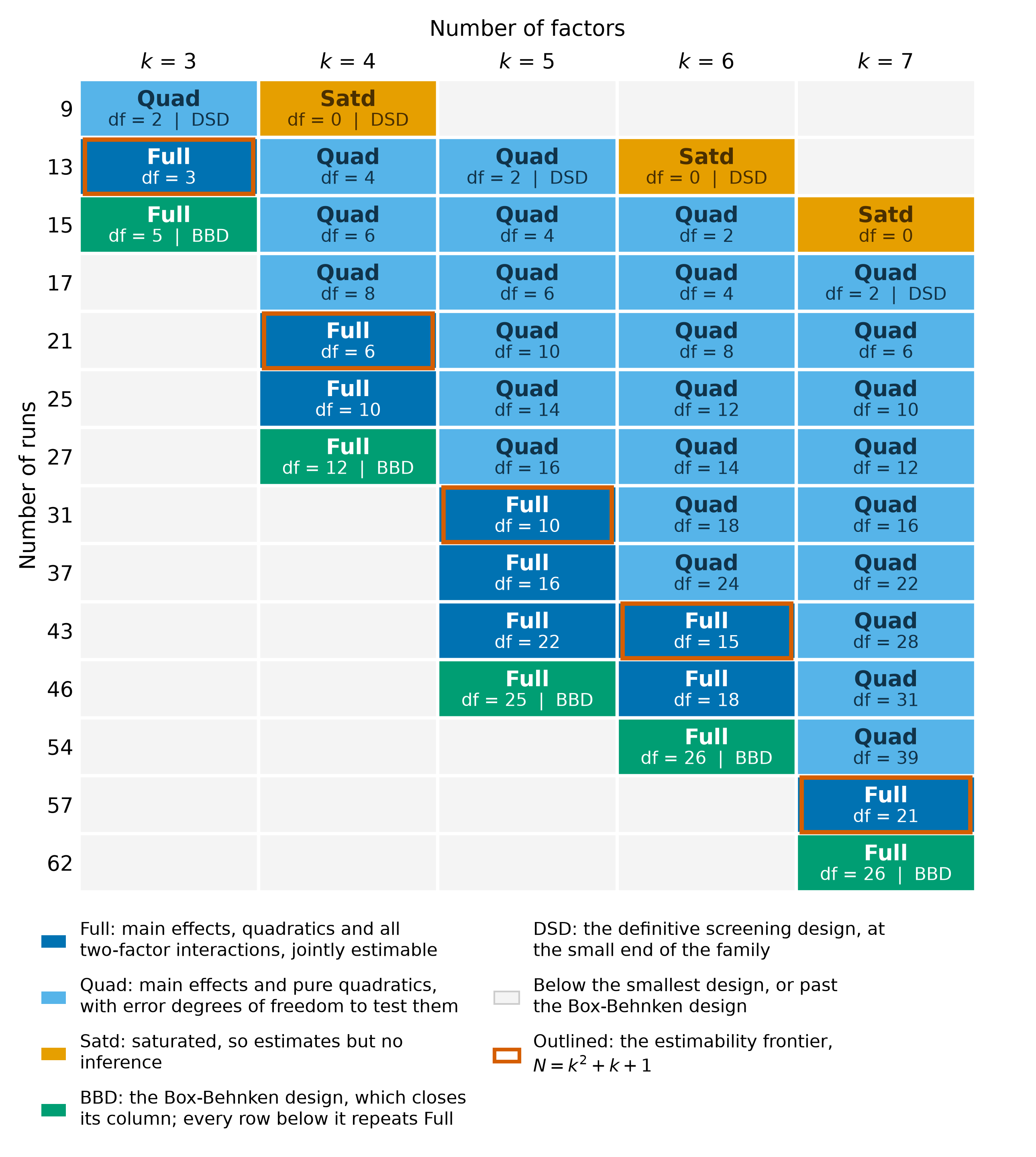
The OMARS trade-off table as a grid of coloured cells, run count down the side and three to seven factors across, each cell labelled Full, Quad or Satd with its error degrees of freedom, the frontier cells outlined and the DSD and Box-Behnken cells marked. — The OMARS trade-off table as a capability staircase. Each cell gives the largest model the run budget makes estimable and the error degrees of freedom left to test it. Outlined cells are the estimability frontier, the first `Full` cell in each column. `DSD` marks the definitive screening design and `BBD`, in green, the Box-Behnken design, each on the row of its run count; the Box-Behnken cell closes its column.¶

The error degrees of freedom are the spare runs left after fitting, which estimate the run-to-run noise \(\sigma^2\) and on which every test and confidence interval rests. Six points to read off the table:

A column runs from about its DSD mark to its BBD mark: the definitive screening design sits at or near the smallest size listed, and the Box-Behnken design is the standard response surface design that closes the column. Below the BBD cell a column is blank, because every further row would say Full again on more runs.

Down a column capability only improves, and across a row it only worsens, so the boundary between the classes is a staircase.

The step up to Full in each column is the estimability frontier: 13, 21, 31, 43 and 57 runs for three to seven factors.

A blank above the BBD mark is a budget below \(2k + 1\), which cannot hold the main effects and the quadratics. The default rows are odd, foldovers with one centre run. The 46- and 54-run rows, added for the Box-Behnken designs, show how an even budget reads: the model of the odd budget one run below, with one more error degree of freedom.

Error degrees of freedom only compare between cells with the same tag, since the tag is what fixes the model being fitted. At 43 runs, six factors show Full df=15 and seven factors show Quad df=28: the seven-factor cell has more spare runs because Quad fits the smaller model, not because it is the better design.

The two marks show what the standard designs cost. For an even number of factors a DSD has \(2k+1\) runs and lands in Satd. For an odd number the conference-matrix construction needs \(2k+3\) runs, so the three-, five- and seven-factor DSDs arrive with two spare degrees of freedom and land in Quad df=2. Every Box-Behnken design is past the frontier and so Full, but none is the smallest design that is: at five factors it takes 46 runs where 31 reach Full.

For a single budget the same information is reported in words, with the neighbouring thresholds:

Output, 6 lines

>>> get_omars_trade_off_table_entry(17, 4)
OMARS: 17 runs, 4 factors
  Quad: main effects and pure quadratics, with error degrees of freedom to test them
  Model: main_quadratic (9 parameters), 8 error df
  Thresholds for 4 factors: Satd 9, Quad 10, Full 21 runs.
  4 more runs would reach Full (all two-factor interactions estimable).

The table carries no quality metrics. D-efficiency, the largest correlation among the second-order effects and the projection properties describe a particular design rather than a size, so they belong to generate_omars and to Judging and comparing designs.

With no run count given, generate_omars sizes the design at the frontier for the model it is asked for:

Python, 5 lines

design = generate_omars([Factor(name=c, low=-1, high=1) for c in "ABCD"], random_state=42)
print(design.n_runs)                                  # 21
print(design.metadata["model_rank"])                  # 15, so the model is estimable
print(design.metadata["min_runs_for_model"])          # 21, the frontier
print(design.metadata["expected_error_df"])           # 6, which is k(k-1)/2

5.16.2.3. Three worked examples¶

Three budgets, read from the table while the design is still a plan. A worked OMARS study then runs one design from plan to recommended recipe.

Six factors in seventeen runs. The cell is Quad df=4: all six main effects and quadratics are estimable, with four degrees of freedom to test them, so curvature can be judged factor by factor. Estimating every interaction jointly takes 43 runs; below that, the staged analysis of Analysing data from these designs selects among them.

Five factors, with a budget that might stretch. Thirteen runs give Quad df=2: estimable and testable, but with two degrees of freedom a 95% confidence interval reaches 4.303 standard errors either side of the estimate. Seventeen runs give Quad df=6, the same model with the multiplier down to 2.447. Thirty-one runs give Full df=10, with every two-factor interaction estimable.

Four factors in nineteen runs, inside the band. That is four runs more than the fifteen parameters of the full second-order model and two short of the frontier. Some quadratics are confounded with interactions, so the full model cannot be fitted; nineteen runs support main effects and pure quadratics, nine parameters with ten error degrees of freedom. None of the data is wasted: the shortfall shows only at the analysis stage.

At twenty-one runs all six interactions join the model, fifteen parameters with six degrees of freedom to test them. Both are sound experiments, so the choice is a budget one: at nineteen runs an interaction that matters has to be found by the staged analysis and confirmed in a follow-up; at twenty-one it arrives with the first design.

5.16.2.4. What a cell in either table reports¶

This section and the next explain the cell contents; the table can be used without them.

A cell of the two-level table gives the best resolution available at its size, not that of every design of that size. Counting every choice of generators gives, for three cells, the number of designs, the best resolution, and how many of the best designs have each number of shortest words in their defining relation:

Python, 24 lines

import functools
import operator
from collections import Counter

def regular_fractions(n_base, n_factors):
    """Resolution and number of shortest words of every regular two-level fraction."""
    columns = [c for r in range(2, n_base + 1)
               for c in itertools.combinations(range(n_base), r)]
    for generators in itertools.combinations(columns, n_factors - n_base):
        words = [frozenset(g) | {n_base + i} for i, g in enumerate(generators)]
        lengths = [len(functools.reduce(operator.xor, subset))
                   for r in range(1, len(words) + 1)
                   for subset in itertools.combinations(words, r)]
        yield min(lengths), lengths.count(min(lengths))

for n_runs, n_factors in ((8, 4), (16, 7), (32, 7)):
    found = Counter(regular_fractions(n_runs.bit_length() - 1, n_factors))
    best = max(resolution for resolution, _ in found)
    at_best = {words: count for (res, words), count in sorted(found.items()) if res == best}
    print(n_runs, n_factors, sum(found.values()), best, at_best)

# 8 4 4 4 {1: 1}
# 16 7 165 4 {7: 4}
# 32 7 325 4 {1: 40, 2: 25, 3: 30}

With eight runs and four factors there are four designs, and only one, \(D = ABC\), reaches resolution IV. Of the 165 sixteen-run, seven-factor designs, four reach resolution IV; with seven four-letter words each, they are one design with the factors relabelled. At 32 runs and seven factors resolution alone does not decide: 95 designs reach resolution IV, and the table prints one with minimum aberration, the fewest four-letter words (Generating the trade-off table). A cell is one design chosen from those that fit the same budget.

The OMARS analogue would be the best quality obtainable at each size. Three properties of the designs, not of any particular measure, stand in the way:

The run count does not fix the design. An OMARS design of \(N\) runs splits its budget between design points and replicates of the centre point. The same twelve design points in three factors, with one, three or five centre runs added, give a largest absolute correlation between second-order terms of \(0.300\), \(0.07143\) and \(0.05556\).
A measure scaled by the run count can get worse as runs are added. The best value of that same correlation is \(0.05556\) at seventeen runs and \(0.1364\) at nineteen.
A measure not scaled by the run count mostly restates it. The alphabetic optimality criteria never worsen when a run is added, but they fall at close to the rate \(1/N\), as Nine measures down one column below shows.

Resolution avoids all three: it is a statement of which effects are confounded with which, not a magnitude, and two-level fractions nest, so extra runs can only break confounding. Neither holds for OMARS designs.

Their cells therefore report a capability class and the error degrees of freedom: statements about estimability, like resolution, and monotone in the run count.

An OMARS cell stands for many more designs than a two-level one: in three factors at twenty-one runs with one centre run there are 1859. The cell says what that budget can estimate; which of the designs to run is a separate choice, made with quality metrics as in An omnibus comparison across design families and Nine measures down one column.

5.16.2.5. Nine measures down one column¶

Could a quality measure be the number in each cell instead? To test this, follow the three-factor column of the OMARS trade-off table down its run counts, plotting at each size the best score any OMARS design of that size reaches: the value a cell would have to report. In three factors every OMARS design of each size can be scored, so these best values are exact.

Write \(\mathbf{M} = \mathbf{X}^T\mathbf{X}\) for the main-effects-and-quadratics model, with \(p = 2k + 1\) terms, and \(\mathbf{f}(\mathbf{x})\) for that model’s row at a point \(\mathbf{x}\) of the region. Six of the nine measures score this model at every run count; five of them are the alphabetic optimality criteria, each a single summary of \(\mathbf{M}\):

\(A/p\), the average coefficient variance. Each fitted coefficient has a variance, the square of the standard error a regression package prints beside it; \(A = \mathrm{tr}(\mathbf{M}^{-1})\) sums those variances and \(A/p\) averages them.
\(D = |\mathbf{M}|^{1/p}\), the joint precision of all \(p\) coefficients at once. The volume of their joint confidence region is proportional to \(|\mathbf{M}|^{-1/2}\), so a larger \(D\) means a smaller region.
\(E = \lambda_{\min}(\mathbf{M})\), the smallest eigenvalue of \(\mathbf{M}\). Some combinations of the coefficients are estimated precisely and others poorly; the worst one has variance \(1/E\), so \(E\) is the worst case matching the average \(A/p\) reports.
\(I = \mathrm{tr}(\mathbf{M}^{-1}\mathbf{B})\), the average prediction variance. A prediction at a setting \(\mathbf{x}\) has variance \(\mathbf{f}^T\mathbf{M}^{-1}\mathbf{f}\), the quantity behind the error band around a fitted curve; \(I\) averages it over the region, with \(\mathbf{B}\) holding the averages of the model terms there.
\(G = \max_{\mathbf{x}}\, \mathbf{f}(\mathbf{x})^T \mathbf{M}^{-1}\mathbf{f}(\mathbf{x})\), the same prediction variance at its worst point in the region, so the worst case matching \(I\).

These are in units of the run-to-run noise: multiplied by \(\sigma^2\), each of \(A/p\), \(I\) and \(G\) is a variance, and its square root is a standard error.

The sixth, max \(|r|\), is not an optimality criterion: it is the largest absolute correlation between any two of the six second-order terms, read off the design’s correlation map.

The remaining three are power: the probability that the test on one coefficient is significant when the coefficient really has a given size. It needs two inputs the six above do not: the effect size \(|\beta|/\sigma\), the coefficient in units of the run-to-run noise, and the significance level \(\alpha\). With coded levels from \(-1\) to \(+1\), \(|\beta|/\sigma = 1\) means a low-to-high change of twice the noise standard deviation. Power also differs by type of term, so each type gets its own plot.

These three plots score the full second-order model, \(p = 1 + 2k + k(k-1)/2\) terms, which the interaction plot needs. So the third row of the figure below starts at thirteen runs, the estimability frontier, while the rows above start at seven or nine.

For a coefficient with variance \(\sigma^2 c\), where \(c\) is its diagonal entry of \(\mathbf{M}^{-1}\), the test statistic follows a non-central \(F\) distribution with \(1\) and \(N - p\) degrees of freedom and non-centrality \(\lambda = (|\beta|/\sigma)^2 / c\). For example, at nineteen runs with one centre run the best attainable \(c\) for a quadratic is 0.2619, so a one-sigma curvature sits \(1/\sqrt{0.2619} = 1.954\) standard errors from zero, against a critical \(t\) of 2.262 at nine degrees of freedom. The test falls short more often than not: the power is 0.4154.

Python, 43 lines

def moment_matrix(k):
    """Moments of the cuboidal region, E[f(x) f(x)'], evaluated exactly."""
    B = np.zeros((2 * k + 1, 2 * k + 1))
    B[0, 0] = 1.0
    for i in range(k):
        B[1 + i, 1 + i] = 1 / 3                                   # E[x_i^2]
        B[0, 1 + k + i] = B[1 + k + i, 0] = 1 / 3
        for j in range(k):
            B[1 + k + i, 1 + k + j] = 1 / 5 if i == j else 1 / 9  # E[x_i^4], E[x_i^2 x_j^2]
    return B

def criteria(levels, grid_levels=7):
    """The five alphabetic criteria for the main-effects-and-quadratics model, and the
    largest absolute correlation between two second-order terms."""
    n_runs, k = levels.shape
    X = np.column_stack([np.ones(n_runs), levels, levels**2])
    M = X.T @ X
    p, M_inv = M.shape[1], np.linalg.inv(M)
    grid = np.array(list(itertools.product(np.linspace(-1, 1, grid_levels), repeat=k)))
    f = np.column_stack([np.ones(len(grid)), grid, grid**2])
    second = [levels[:, i] ** 2 for i in range(k)]
    second += [levels[:, i] * levels[:, j] for i, j in itertools.combinations(range(k), 2)]
    C = np.abs(np.corrcoef(np.column_stack(second), rowvar=False))
    return {"A/p": np.trace(M_inv) / p,
            "D": np.linalg.det(M) ** (1 / p),
            "E": np.linalg.eigvalsh(M).min(),
            "I": np.trace(M_inv @ moment_matrix(k)),
            "G": ((f @ M_inv) * f).sum(axis=1).max(),
            "max |r|": C[~np.eye(len(C), dtype=bool)].max()}

# The twelve design points behind the centre-run example in the first obstacle, as six half-rows
# and their negations, scored with one, three and five centre runs added.
half = np.array([[0, 1, -1], [0, 1, 1], [1, -1, 0],
                 [1, 0, -1], [1, 0, 1], [1, 1, 0]], dtype=float)
points = np.vstack([half, -half])
for n_centre in (1, 3, 5):
    levels = np.vstack([points, np.zeros((n_centre, 3))])
    values = criteria(levels)
    print(f"N = {len(levels)}   " + "   ".join(f"{n} = {v:#.4g}" for n, v in values.items()))

# N = 13   A/p = 0.3839   D = 5.384   E = 0.5626   I = 0.5125   G = 1.000   max |r| = 0.3000
# N = 15   A/p = 0.2173   D = 6.298   E = 1.635   I = 0.3014   G = 0.6458   max |r| = 0.07143
# N = 17   A/p = 0.1839   D = 6.775   E = 2.635   I = 0.2592   G = 0.6125   max |r| = 0.05556

Power is computed from the same design, against the full second-order model:

Python, 25 lines

from scipy import stats

def power(levels, effect_size=1.0, alpha=0.05):
    """Power for a main effect, an interaction and a quadratic, full second-order model."""
    n_runs, k = levels.shape
    pairs = list(itertools.combinations(range(k), 2))
    X = np.column_stack([np.ones(n_runs), levels, levels**2]
                        + [levels[:, i] * levels[:, j] for i, j in pairs])
    df = n_runs - X.shape[1]
    c = np.diag(np.linalg.inv(X.T @ X))
    blocks = {"main effect": c[1:k + 1],
              "interaction": c[2 * k + 1:],
              "quadratic": c[k + 1:2 * k + 1]}
    critical = stats.f.ppf(1 - alpha, dfn=1, dfd=df)
    return {name: 1 - stats.ncf.cdf(critical, dfn=1, dfd=df,
                                    nc=effect_size**2 / block.max())
            for name, block in blocks.items()}

# The same twelve points with three centre runs: the Box-Behnken design in three factors.
for term, value in power(np.vstack([points, np.zeros((3, 3))])).items():
    print(f"{term:>12} {value:#.4g}")

#  main effect 0.6228
#  interaction 0.3682
#    quadratic 0.3450

Factorial, the designed-experiments app, computes the same nine measures in the browser, for factors a reader enters and every design the app can generate for them.

Running criteria and power on every OMARS design of every size in three factors, and keeping the best value of each measure at each size, gives the nine curves below.

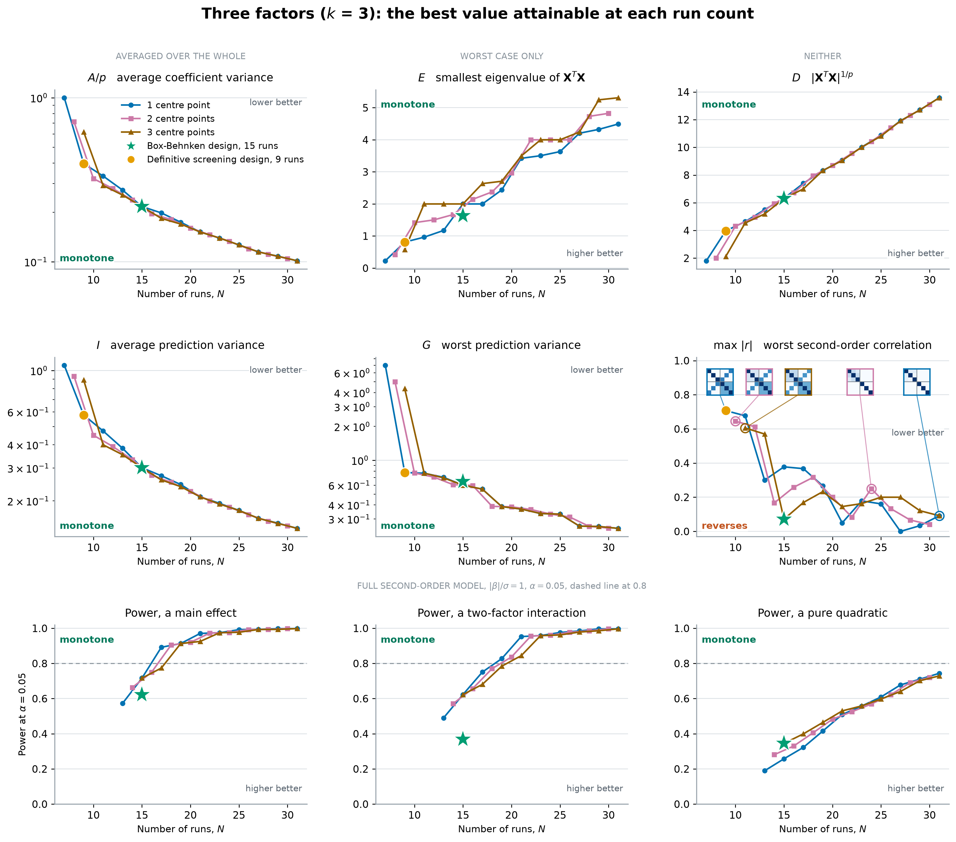
Nine small plots of design measures against run count for three factors: A/p, I, D, E, G and max |r| in the first two rows and power for a main effect, an interaction and a quadratic in the third, with correlation-map insets. — Nine candidate measures down the three-factor column of the OMARS trade-off table, each point the best value attainable at that run count over every OMARS design of the size. In the first two rows the left pair of plots averages, the middle pair takes the worst case of the same two quantities, and the right pair does neither. The insets are correlation maps of five plotted designs, rows and columns the three quadratics then the three interactions, darker squares for higher correlation on a common scale from zero to one; each is outlined in its series’ colour, and the three on the left are the smallest design at each centre-run count. The third row is power for each type of term, scoring the full second-order model. The nine-run definitive screening design is an orange circle and the fifteen-run Box-Behnken design a green star, the colours they carry in the trade-off table.¶

Read together, the plots make these points:

\(A/p\), \(I\) and \(D\) restate the run count. \(A/p\) and \(I\) fall at close to the rate \(1/N\), so the product \(N \times A/p\) is nearly constant down the column. \(D\) rises almost in a straight line, and the three centre-run series nearly coincide.
\(E\) rises as a staircase with flat treads. Along a tread, the extra runs do not improve the combination of coefficients the data estimate worst.
\(G\) has a floor that no design can beat. Kiefer and Wolfowitz showed that no design of \(N\) runs has \(G\) below \(p/N\), and the best three-factor designs touch that floor at a few sizes.
Max \(|r|\) can get worse as runs are added, and it separates the centre-run series widely. The three insets on the left show why: the same design points with more centre runs have a lower correlation between a quadratic and an interaction, but a higher one between two quadratics. Among the designs in the figure, it reaches zero only for the full three-level factorial at twenty-seven runs; the same twelve points with four centre runs reach it at sixteen.
Power rises steadily with the run count, like the alphabetic criteria, and it ranks the types of term. Main effects need the fewest runs, interactions a few more, and quadratics far more. An interaction column takes the values \(\pm 1\), like a main effect, while a quadratic column takes only zero and one and overlaps the intercept. The quadratics therefore set the run count.
Centre runs trade one kind of power for another. They lower main-effect and interaction power and raise quadratic power, up to about twenty-five runs.
The nine-run definitive screening design is the best design of its size on all six measures of the first two rows. It has nine runs rather than \(2k + 1 = 7\) because its conference matrix needs an even order, so three factors use one of order four and drop a column.
The fifteen-run Box-Behnken design reaches the best attainable value for five measures and falls short of it for four. Its runs sit on the edges of the cube rather than the corners, which favours curvature over main effects, interactions and the worst-case measures \(E\) and \(G\).
The measures disagree about which design is best. At twenty-one runs with one centre run there are 1859 OMARS designs, and the six measures of the first two rows pick four different ones. A single number in a cell would have to say which measure it is.
Power is not a single number either. It needs an effect size and a significance level, gives a separate value for each type of term, and changes with the model being scored.

The two tools therefore divide the work. The trade-off table sets the run count from capability and error degrees of freedom; at that run count, candidate designs are compared on the measure that matches the aim of the study: \(A\) or \(E\) for precise coefficients, \(I\) or \(G\) for prediction over the region, max \(|r|\) for keeping the second-order effects apart, or power for detecting an effect of a stated size.

5.16.2.6. The same measures with four factors¶

These conclusions do not depend on there being three factors. The four-factor column, drawn the same way in the figure below, reads the same: the alphabetic criteria never get worse as runs are added, the best attainable max \(|r|\) still can, and the power row cannot start before the estimability frontier at 21 runs.

Every four-factor design up to 21 runs, a ten-row half-design folded over plus a centre run, was scored (up to 22 and 23 runs with two and three centre runs). Beyond that there are too many designs of each size to score them all, so those points are the best design a search found, a bound on what is attainable rather than the best value itself. On the sizes where both are available, the search found the exact best every time.

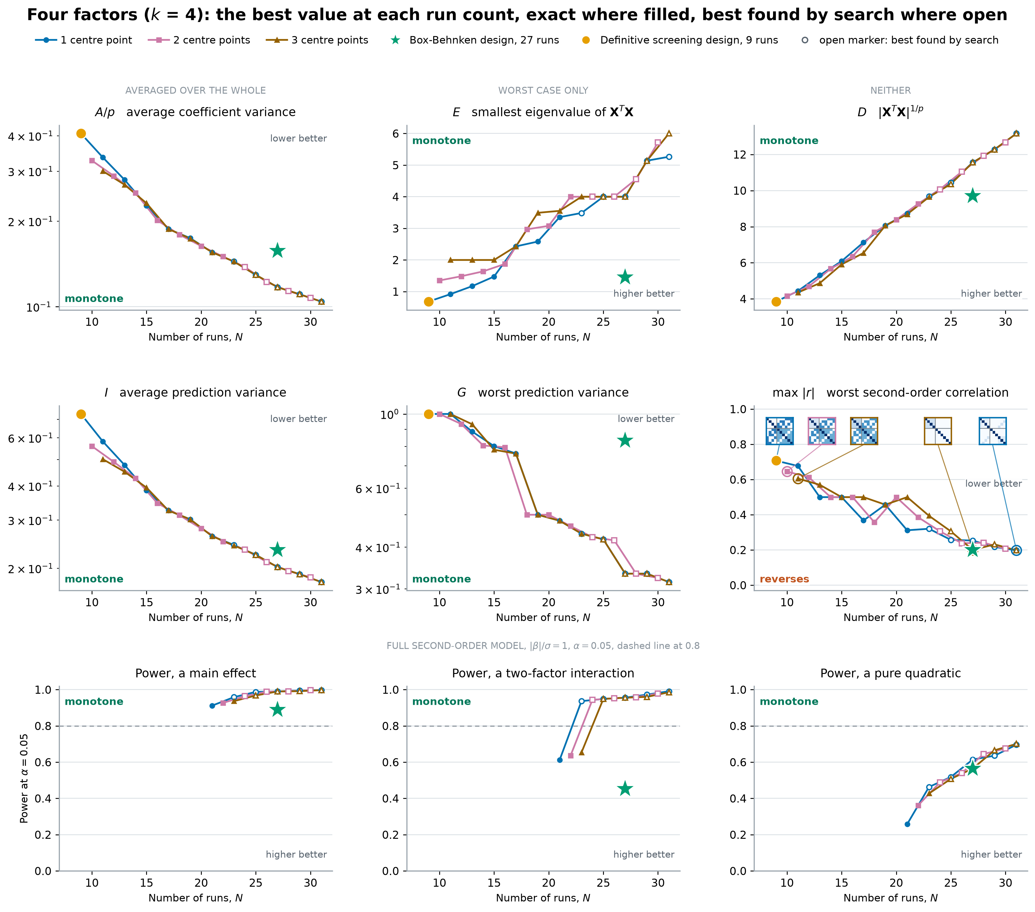
The nine plots of design measures against run count, as in the three-factor figure, for four factors, with filled markers for exact values and open markers for values found by search. — The nine measures of the three-factor figure, for the four-factor column of the OMARS trade-off table. Filled markers are the best value over every OMARS foldover of that size; open markers, for the larger designs, are the best design found by search. The nine-run definitive screening design is an orange circle and the 27-run Box-Behnken design a green star.¶

5.16.3. Analysing data from these designs¶

Data from these designs call for an analysis that uses their structure, rather than a least-squares fit of the full second-order model or a generic search over all its terms.

The full model is often not estimable. In four factors it has \(1 + 4 + 4 + 6 = 15\) terms, more than a nine-run DSD or a thirteen-run OMARS design provides, and as the estimability frontier shows, a nineteen-run foldover cannot estimate them either.

A generic stepwise or penalised regression leaves the main effects unbiased, since the design makes them orthogonal to every second-order column, but it searches all the columns together. Its error estimate absorbs any active second-order effect it leaves out, and it treats correlated second-order terms as though they were not. In simulations by Hameed, Núñez Ares and Goos (2023), the staged analysis below detected active effects more often than stepwise regression, the Dantzig selector and hierNet, while keeping false detections under control.

This design-based analysis works in stages: estimate the main effects, which the design keeps clean; pool the inactive ones into the error estimate; then test for, and select among, the second-order effects in their own subspace, limited by how few can be told apart:

Code, 29 lines

design matrix  +  measured responses
         |
         v
(0)  is the model ESTIMABLE, with error df to spare?
     ( rank of the model matrix equals the number of terms
       being fitted, and the run count exceeds it )
     if not  ->  stop; shrink the model, replicate, or add runs
         |
         v
(1)  estimate the MAIN EFFECTS
     clean and unbiased: they are orthogonal to every
     second-order term, whichever of those are active
         |
         v
(2)  test them; pool the INACTIVE effects back into the
     error estimate, recovering degrees of freedom
         |
         v
(3)  one F-TEST: is any second-order effect active at all?
     if not  ->  report the main-effects model
         |
         v
(4)  SELECT the active second-order effects, limited by how
     many are jointly estimable, and optionally guided by
     effect heredity ( an interaction is admitted only if its
       parent main effects are active )
         |
         v
final model: the active main, quadratic, and interaction effects

Steps 0 and 4 need explanation; step 1 rests on the orthogonality the design guarantees.

Step 0 checks that the analysis can start. A saturated design leaves nothing to estimate \(\sigma^2\), and in a foldover below the estimability frontier the coefficients have no unique solution, which is why the check is on the rank of the model matrix, not the run count.

Step 4 manages the design’s one weakness: the second-order effects are correlated among themselves, so only a limited number can be estimated together.

The procedure is that of Jones and Nachtsheim (2017) for definitive screening designs, extended to OMARS designs by Hameed, Núñez Ares and Goos (2023). In process_improve it is analyze_omars(), which accepts any design in two- or three-level quantitative factors, though its stages assume the main effects are orthogonal to the second-order terms. It tests the main effects at 5% and the second-order terms at 20%, the levels Hameed et al. use, and returns the result of each stage.

Heredity in step 4 is an option, not the default. With interaction_heredity="none" and quadratic_heredity="none" every quadratic and interaction is a candidate, and a best-subset search adds terms until the remaining second-order variation is no longer significant. The other settings are:

interaction_heredity="strong", the rule in the diagram: an interaction is admitted only if both of its parent main effects are active.
interaction_heredity="weak": at least one parent main effect must be active.
quadratic_heredity="strong": a quadratic is admitted only if its own main effect is active.

Heredity can mislead in either direction. When a factor’s optimum lies near the centre of its range its linear effect is small, so strong heredity can drop the terms that locate the optimum, as A worked OMARS study shows on a simulated bioreactor. Without heredity, the search can admit an interaction that knowledge of the process rules out, as Goos, Núñez Ares, Hameed and Lanzerath (2026) report for a polymerization experiment. Comparing the models under each setting shows which conclusions depend on the choice.

Goos et al. (2026) also refit each selected model with the main effect of every factor in its second-order terms, a convention called model marginality. All-subset regression by mixed-integer optimisation (Vazquez, Schoen and Goos, 2021) takes a different route, listing many well-fitting models and comparing the terms they share in a raster plot.